James-Stein estimator

James-Stein estimator set-up

Suppose that we’re interested in estimating \(K\) independent means collected into a vector \(\boldsymbol{\theta}\), about which we observe a normally distributed RV \(\mathbf{X}\), with realization \(\mathbf{x}\)

\[ \mathbf{X} \mid \boldsymbol{\theta} \sim \text{MultiNormal}(\boldsymbol{\theta}, I_K) \]

We’ll measure the quality of an estimator for \(\boldsymbol{\theta}\), \(\boldsymbol{\delta}(\mathbf{x})\) with a function \(L(\boldsymbol{\theta}, \boldsymbol{\delta}(\mathbf{x}))\) \[ L(\boldsymbol{\theta}, \boldsymbol{\delta}(\mathbf{x})) = \sum_{k=1}^K (\boldsymbol{\theta}_k - \boldsymbol{\delta }_k(\mathbf{x}))^2 \]

We can compare estimators at a given \(\boldsymbol{\theta}\) by taking expectations of \(L(\boldsymbol{\theta}, \boldsymbol{\delta}(\mathbf{X}))\) over \(\mathbf{X} \sim \text{MultiNormal}(\boldsymbol{\theta}, I_K)\)

\[ R(\boldsymbol{\theta}, \mathbf{\delta}) = \Exp{L(\boldsymbol{\theta}, \boldsymbol{\delta}(\mathbf{X}))} \]

James and Stein (1961) show that the “usual estimator” \(\boldsymbol{\delta}^\text{usual}(\mathbf{x}) = \mathbf{x}\) has uniformly (i.e. for all \(\boldsymbol{\theta}\)) higher risk than \(\boldsymbol{\delta}^{\text{JS}}(\mathbf{x})\)

\[ \delta^{\text{JS}}(\mathbf{x}) = \lp 1 - \frac{K-2}{\sum_{k=1}^K \mathbf{x}_k^2} \rp \mathbf{x} \]

Intuition behind Stein estimator

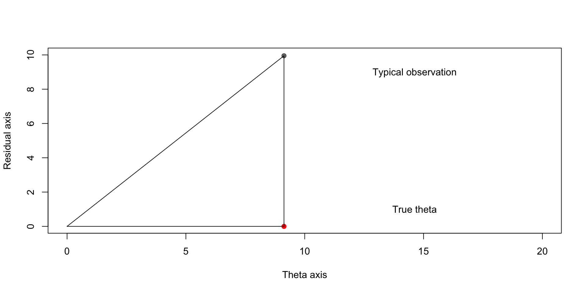
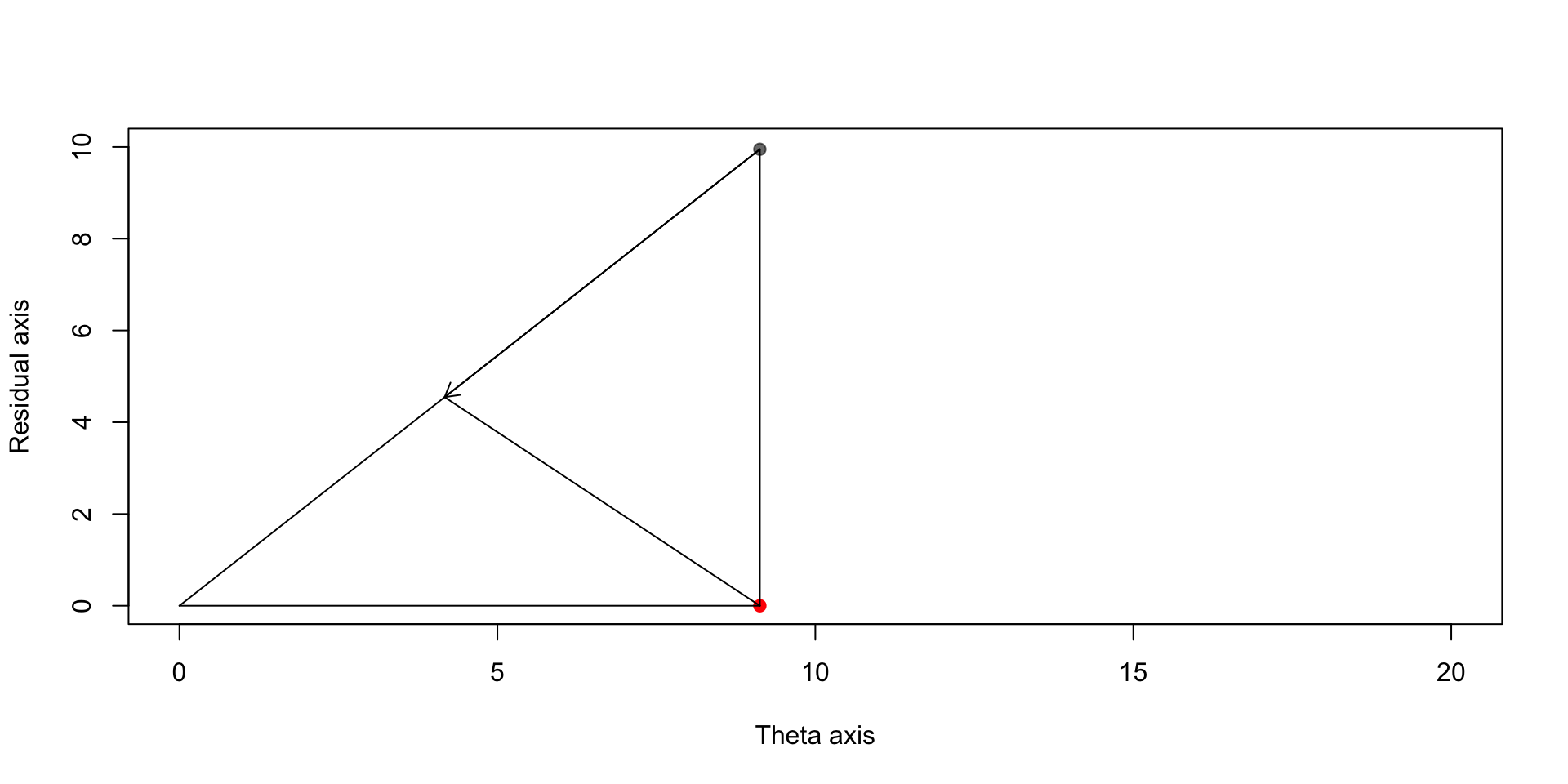
Brown and Zhao (2012) works through the geometric intuition behind the estimator.

It requires that we change our basis for \(\R^K\) from the standard basis to a basis in which one vector is pointed in the direction of \(\boldsymbol{\theta}\), and the rest are orthogonal to that direction.

The way we would do that is to do something like:

set.seed(123)
theta <- rnorm(10)
trans_mat <- cbind(theta, diag(10)[,-1])

basis_mat <- qr.Q(qr(trans_mat))
manual_basis <- theta / sqrt(sum(theta^2))
sum(abs(basis_mat[,1] - manual_basis))

[1] 3.712308e-16

theta_in_new_basis <- t(basis_mat) %*% theta
red_theta <- c(theta_in_new_basis[1], sqrt(sum(tail(theta_in_new_basis^2,-1))))
red_theta

[1] 2.871067e+00 7.393830e-16

X <- theta + rnorm(10)
X_in_new_basis <- t(basis_mat) %*% X
red_X <- c(X_in_new_basis[1], sqrt(sum(tail(X_in_new_basis^2,-1))))
plot(red_theta[1],0, xlim = c(0,5), ylim = c(0,5),
     xlab = "Theta axis", ylab = "Residual axis",
     col = "red", pch = 19)
Xs <- sweep(matrix(rnorm(1e4), 10, 1e3), 1, theta, FUN = "+")
trans_Xs <- t(basis_mat) %*% Xs
trans_Xs_red <- cbind(trans_Xs[1,], sqrt(colSums(trans_Xs[2:10,]^2)))
points(trans_Xs_red[,1], trans_Xs_red[,2],pch = 19, col = scales::alpha("black",0.6))

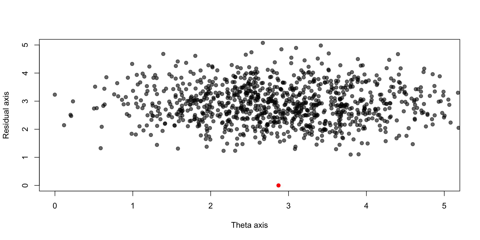
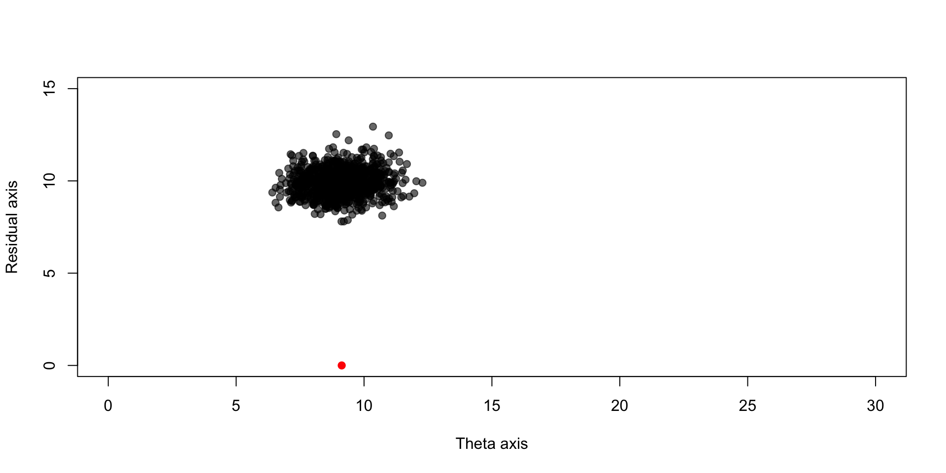
The point cloud is shifted above the true theta; this shift gets worse as dimension of \(\boldsymbol{\theta}\) increases

Why does the cloud shift up?

Explaining why the cloud shifts up as \(K\) increases requires a bit of normal theory

Recall that for a multivariate normal RV \(\mathbf{X}\) with parameters \(\boldsymbol{\theta}\) and \(I_K\), \(A^T \mathbf{X}\) is again multivariate normal with mean \(A\boldsymbol{\theta}\) and covariate \(A^T A\).

The transformation we’ve done is \(Q^T \mathbf{X}\) where \(Q^T Q = I_K\). Thus \(Q^T \mathbf{X} \sim \text{MVN}(Q^T \boldsymbol{\theta}, I_K)\)

The way we’ve represented \(Q^T \mathbf{X}\) is by the first coordinate \(Q_1^T \mathbf{X}\) and the 2-norm of the last \(K-1\) elements:

\[ \lp Q_1^T \mathbf{X}, \sqrt{\sum_{k=2}^K (Q_k^T \mathbf{X})^2}\rp \]

The RVs \(Q_k^T \mathbf{X}\) are independent mean-zero normal RVs, a sum of \(K-1\) squared normal RVs is chi-squared \(K - 1\)

\[ Q^T_k (\boldsymbol{\theta} + \mathbf{Z}) = Q^T_k\mathbf{Z}, k > 1 \]

James-Stein estimator

Ideally we would like to shrink our estimators toward \(\boldsymbol{\theta}\), but in the absence of knowledge of this point, we can shrink toward the origin:

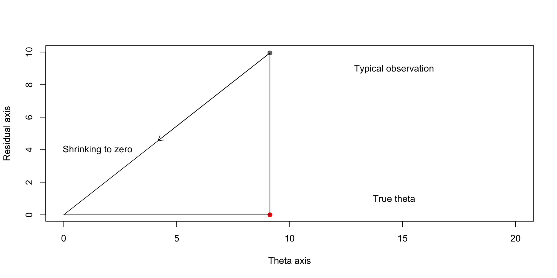
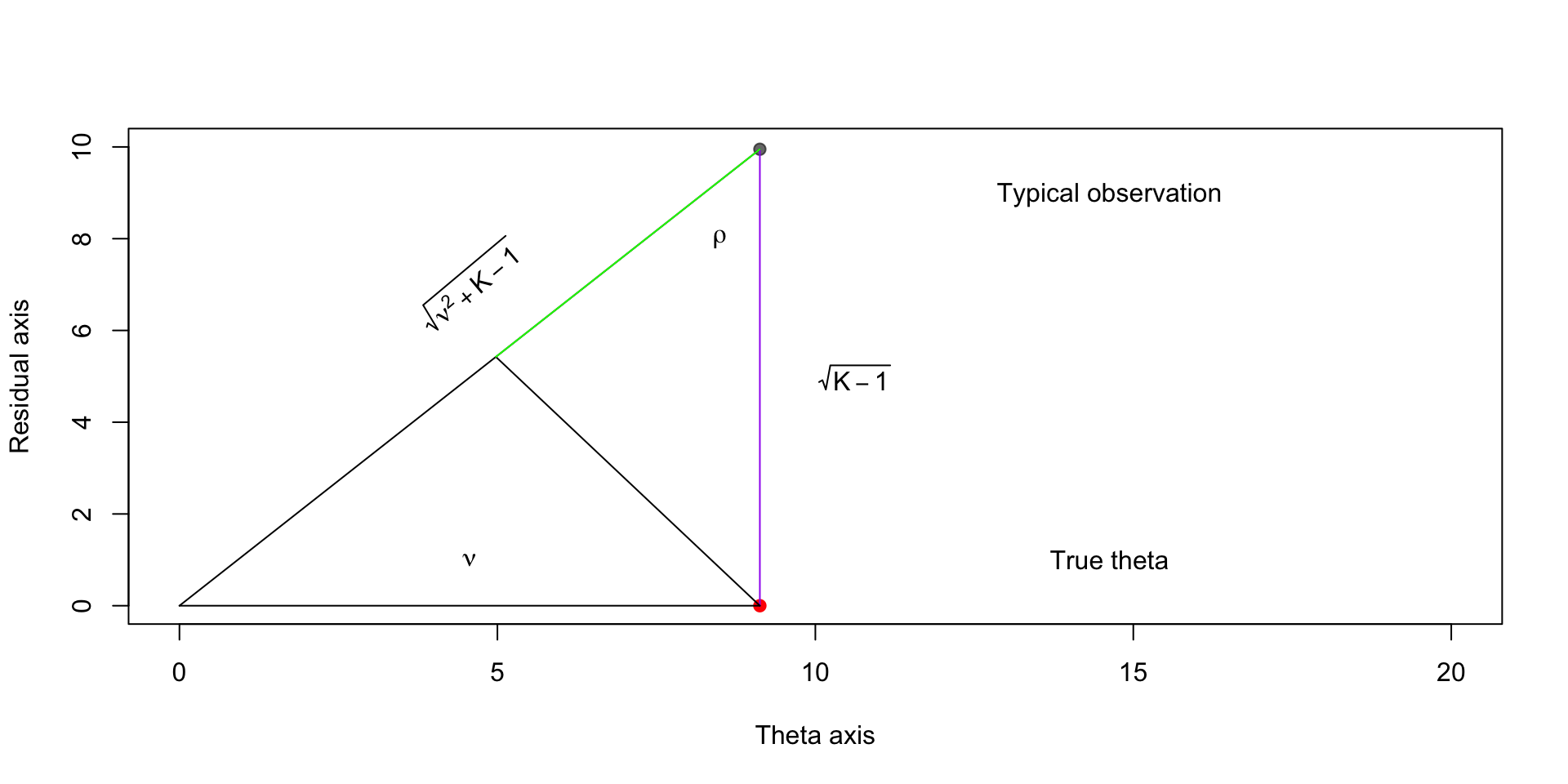
Finding the optimal shrinkage

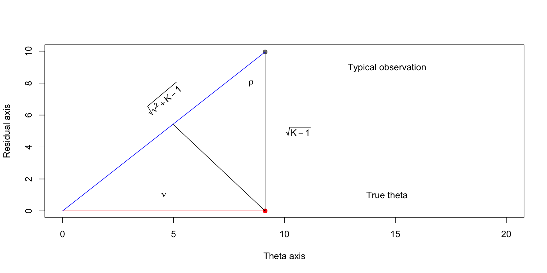
\[ \begin{aligned} \sin \rho & = \frac{\textcolor{red}{\nu}}{\textcolor{blue}{\sqrt{\nu^2 + K - 1}}} \end{aligned} \]

\[ \begin{aligned} \sin \rho & = \frac{\textcolor{green}{y}}{\textcolor{purple}{\sqrt{K - 1}}} \end{aligned} \]

Implies that \(y = \sqrt{K - 1} \frac{\nu}{\sqrt{\nu^2 + K - 1}}\)

Compare this to \(\sqrt{K-1}\), which is how far away the typical observation is

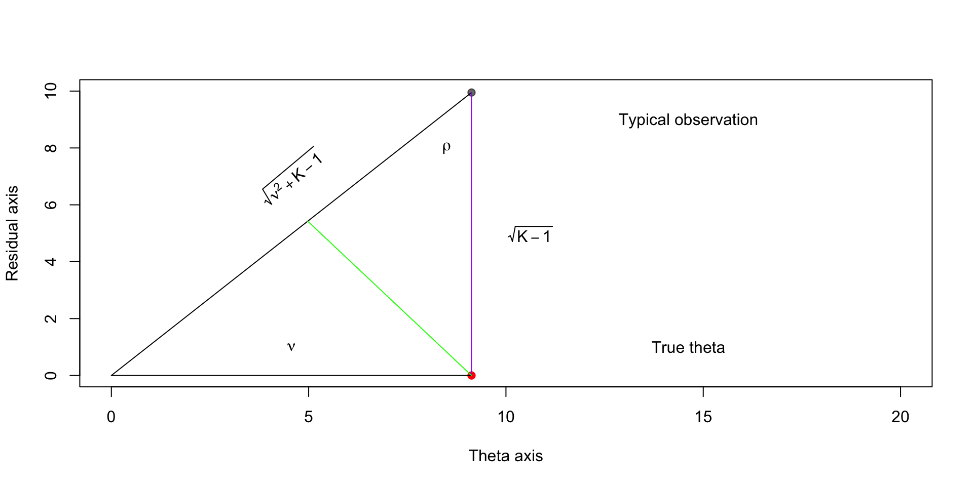
Finding the optimal estimator

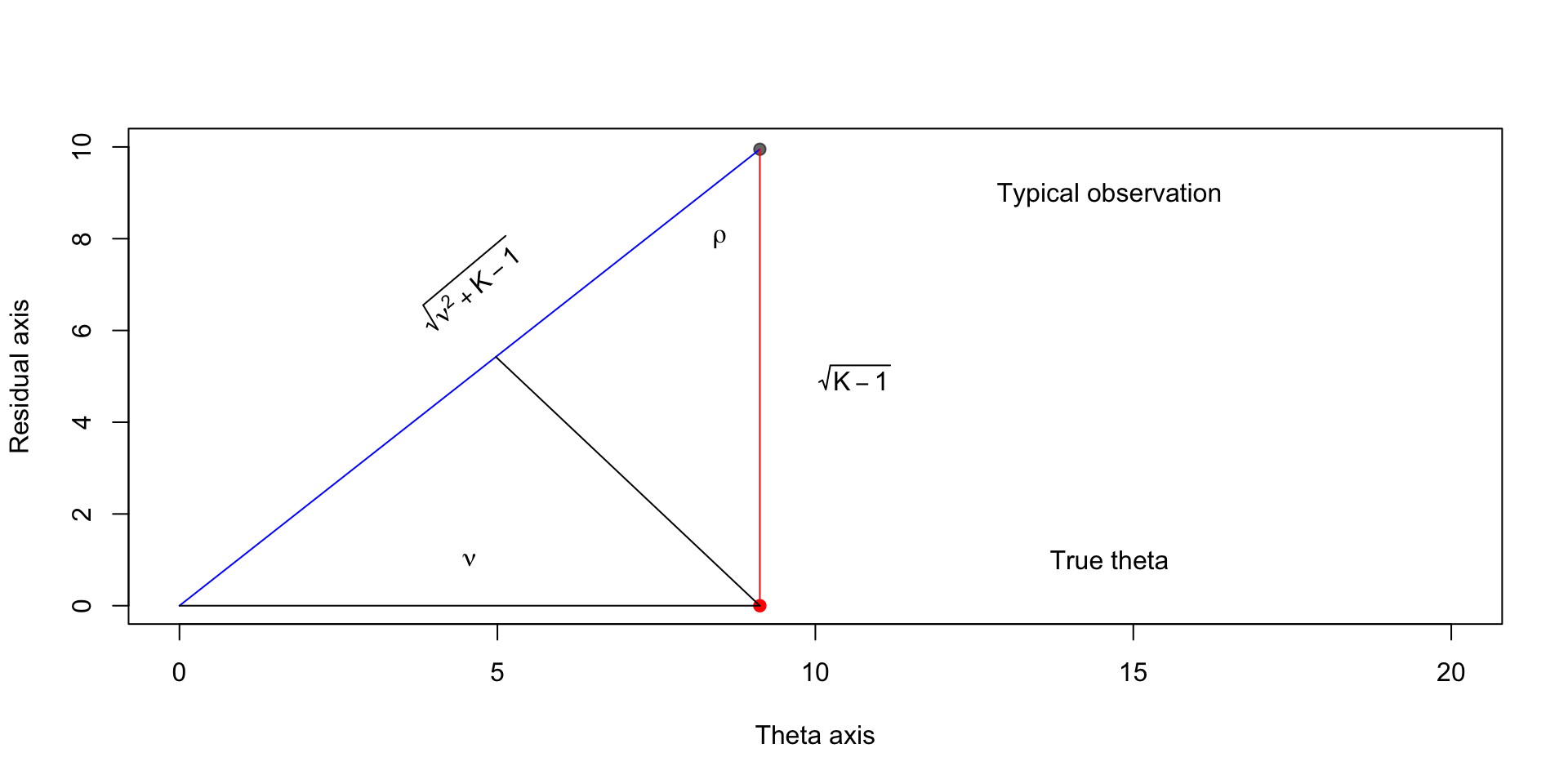
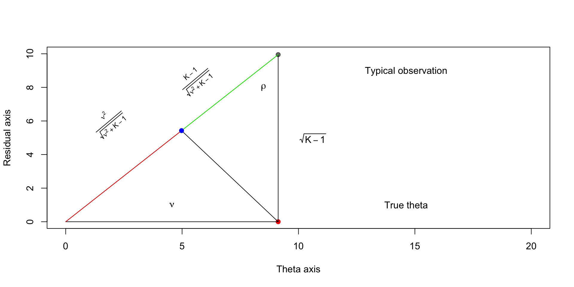
\[ \begin{aligned} \cos \rho & = \frac{\textcolor{red}{\sqrt{K-1}}}{\textcolor{blue}{\sqrt{\nu^2 + K - 1}}} \end{aligned} \]

\[ \begin{aligned} \cos \rho & = \frac{\textcolor{green}{y}}{\textcolor{purple}{\sqrt{K - 1}}} \end{aligned} \]

Implies that \(y = \frac{K - 1}{\sqrt{\nu^2 + K - 1}}\).

This means that we shrink the point \((\nu, \sqrt{K-1})\) to the origin by the amount \(\lp 1 - \frac{K - 1}{\nu^2 + K - 1}\rp\)

Then the estimator in this new basis is \[ \lp 1 - \frac{K - 1}{\nu^2 + K - 1}\rp\begin{bmatrix} \nu \\ \sqrt{K - 1} \end{bmatrix} \]

Moving back to the original basis

Recall that \((\nu, \sqrt{K-1})\) is a “typical” point \(Q^T \mathbf{X}\), or \((Q_1^T \mathbf{X}, \sqrt{\sum_{k=2}^K (Q_k^T \mathbf{X}})^2)\)

The norm of \((Q_1^T \mathbf{X}, \sqrt{\sum_{k=2}^K (Q_k^T \mathbf{X}})^2)\) is \(\sqrt{\sum_{k=1}^K (Q_k^T \mathbf{X})^2}\)

We can write this in matrix notation as \(\mathbf{X}^T Q Q^T\mathbf{X}\)

Then

\[ \begin{aligned} \mathbf{X}^T Q Q^T\mathbf{X} & = \mathbf{X}^T \mathbf{X} \end{aligned} \]

Then \[ \lp 1 - \frac{K - 1}{\nu^2 + K - 1 } \rp = \lp 1 - \frac{K - 1}{\mathbf{X}^T \mathbf{X} } \rp \]

This implies

\[ \lp 1 - \frac{K - 1}{\mathbf{X}^T \mathbf{X} } \rp \mathbf{X} \] is optimal from a geometric standpoint

The factor of \(K-1\) in the numerator is not quite right, and the \(K-2\) found in the James-Stein estimator can be motivated by an empirical Bayes argument.

Key intuition from shrinkage estimation

When estimating \(\boldsymbol{\theta}\) from \(\mathbf{X} \sim \text{MVN}(\boldsymbol{\theta}, I_K)\), \[\norm{\mathbf{X}}^2 = \norm{\boldsymbol{\theta}}^2 + p + O_p(\sqrt{p})\]

So \(\norm{\boldsymbol{\theta}} = \sqrt{\norm{\mathbf{X}}^2 - p - O_p(\sqrt{p})}\) or

\[\norm{\boldsymbol{\theta}} \approx \norm{\mathbf{X}} \lp 1 - \frac{p + O_p(\sqrt{p})}{2\norm{\mathbf{X}}^2} \rp\]

The norm of \(\mathbf{X}\) is likely to be too large by a factor of approximately \(p\), so we should shrink \(\mathbf{X}\)

“Empirical” Bayes derivation

An alternative derivation of the James-Stein estimator can be motivated by a quasi-Bayesian argument, which is otherwise known as “empirical Bayes” estimation

Suppose \[ \begin{aligned} \boldsymbol{\theta} & \sim \text{Normal}(0, b^2 I_K) \\ \mathbf{X} \mid \boldsymbol{\theta} & \sim \text{Normal}(\boldsymbol{\theta}, I_K) \end{aligned} \]

Then for fixed \(b\), we just have a collection of univariate normal posteriors, where the posterior mean for \(\boldsymbol{\theta}_k\) is \[ \mathbf{X}_k \frac{b^2}{b^2 + 1} = \mathbf{X}_k\lp 1 - \frac{1}{b^2 + 1} \rp \]

We don’t know \(b\), so we need to estimate it from the data. One approach is to come up with an unbiased estimator for \((b^2 + 1)^{-1}\)

Marginalizing over \(\boldsymbol{\theta}\), we get that \[ \begin{aligned} \mathbf{X} & \sim \text{Normal}(\mathbf{0}, (b^2 + 1)I_K) \end{aligned} \]

We know the distribution for \[\frac{S^2}{b^2 + 1} = \sum_{k=1}^K \lp\frac{\mathbf{X}_k}{\sqrt{b^2 + 1}}\rp^2\]

\[ \frac{S^2}{b^2 + 1} \sim \text{Chi-squared}(K) \]

Implies that \((b^2 + 1) / S^2\) is inverse chi-square and \(\Exp{(b^2 + 1) / S^2} = \frac{1}{K - 2}\)

Then \[ \begin{aligned} \frac{K-2}{b^2 + 1}\Exp{(b^2 + 1) / S^2} & = \frac{1}{b^2 + 1}\\ \Exp{K - 2 / S^2} & = \frac{1}{b^2 + 1} \end{aligned} \]

Putting it all together \[ \Exp{\boldsymbol{\theta}_k \mid \mathbf{X}_k} = \mathbf{X}_k\lp 1 - \frac{K - 2}{\mathbf{X}^T \mathbf{X}} \rp \]

Shrinking to a different mean

We don’t have to shrink to zero; we can instead shrink to an arbitrary \(\mu\)

\[ \delta^{\mathrm{JS}}(\mathbf{x}) = \boldsymbol{\mu} + \lp 1 - \frac{K - 2}{(\mathbf{X} - \boldsymbol{\mu})^T (\mathbf{X} - \boldsymbol{\mu})}\rp(\mathbf{X} - \boldsymbol{\mu}) \]

Surpisingly, this has the same risk as the original James-Stein estimator that shrinks to the origin, albeit with a translation of \(\mathbf{X}\): \[ R(\boldsymbol{\theta},\boldsymbol{\delta}^{\mathrm{JS}}) = K - (K - 2)^2 \Exp{\frac{1}{(\mathbf{X} - \boldsymbol{\mu})^T (\mathbf{X} - \boldsymbol{\mu})}} \]

This estimator still dominates \(\mathbf{X}\) in terms of risk, but its benefit over the MLE diminishes the farther \(\mathbf{\mu}\) is from \(\boldsymbol{\theta}\), the true mean of \(\mathbf{X}\)

Hierarchical Bayes

Suppose we have the following hierarchical model for \(\boldsymbol{\theta}\): \[ \begin{aligned} X_i \mid \theta_i & \overset{\text{iid}}{\sim} \text{Normal}(\theta_i, 1), i = 1, \dots, K \\ \theta_i \mid \mu, \tau & \sim \text{Normal}(\mu, \tau^2) \\ \mu & \sim \text{Normal}(a, b^2)\\ \tau & \sim p(\tau) \end{aligned} \]

Our posterior mean given \(\tau\) can be expressed: \[ \mathbf{X}_i - \frac{1}{1 + \tau^2}(\mathbf{X}_i - \bar{\mathbf{X}}) - \frac{1}{pb^2 + 1 + \tau^2}(\bar{\mathbf{X}} - a) \]

Comparing priors for normal-normal model

The posterior mean under the normal-normal model

\[ \begin{aligned} X_i \mid \theta_i & \overset{\text{iid}}{\sim} \text{Normal}(\theta_i, 1), i = 1, \dots, K \\ \theta_i \mid \tau_i & \sim \text{Normal}(0, \tau_i^2) \\ \tau_i & \sim p(\tau) \end{aligned} \]

can be expressed as \[ \Exp{\theta_i \mid \mathbf{x}} = \int_0^\infty \left(1 - \frac{1}{1 + \tau_i^2}\right) \mathbf{x}_i\, p(\tau_i \mid \mathbf{x}) d\tau_i \]

We can transform variables from \(\tau_i \in (0,\infty)\) to \(\kappa_i = \frac{1}{1+\tau_i^2} \in (0,1)\):

\[ \Exp{\theta_i \mid \mathbf{x}} = \int_{0}^1 (1 - \kappa_i)\mathbf{x}_i p(\kappa_i \mid \mathbf{x}) d\kappa_i \]

or

\[ \Exp{\theta_i \mid \mathbf{x}} = (1 - \Exp{\kappa_i \mid \mathbf{x}})\mathbf{x}_i \]

Thus, we can compare priors for \(\tau_i\) by comparing the densities of \(\kappa_i\)

Examples of priors for normal-normal

Strawderman proposes a proper Bayesian model that minimizes maximum risk:

\[ \begin{aligned} X_i \mid \theta_i & \overset{\text{iid}}{\sim} \text{Normal}(\theta_i, 1), i = 1, \dots, K \\ \theta_i \mid \lambda & \sim \text{Normal}(0, (1 - \lambda)/\lambda) \\ \lambda & \sim \text{Unif}(0,1) \end{aligned} \]

The horseshoe prior, and its variants are a more recent addition to shrinkage estimators

\[ \begin{aligned} X_i \mid \theta_i & \overset{\text{iid}}{\sim} \text{Normal}(\theta_i, 1), i = 1, \dots, K \\ \theta_i \mid \lambda_i & \sim \text{Normal}(0, \lambda_i^2) \\ \lambda_i \mid \tau & \sim \text{Cauchy}^+(0,\tau) \\ \tau & \sim \text{Cauchy}^+(0, 1) \end{aligned} \]

Plots of \(\kappa_i\) for different shrinkage priors

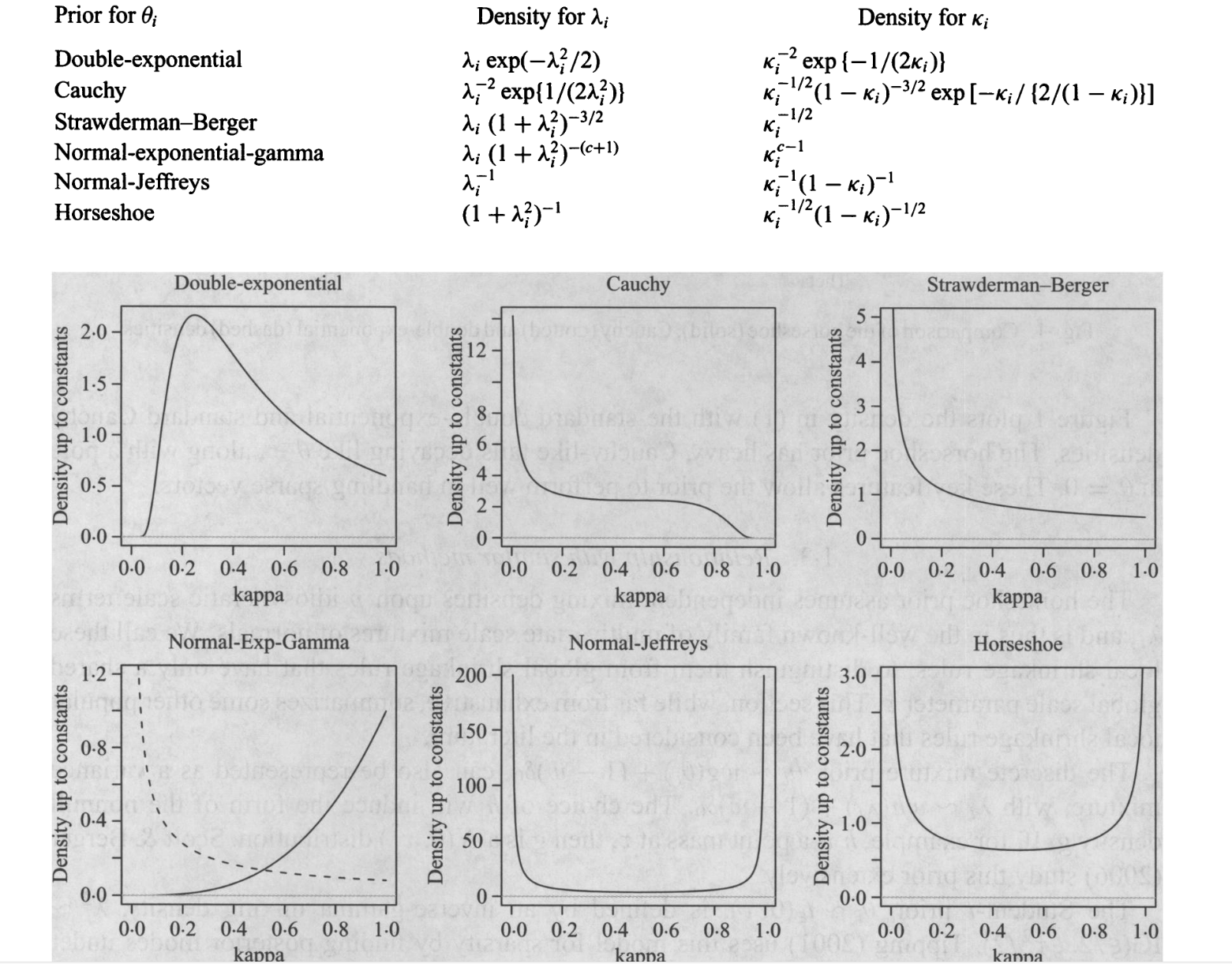
Shrinkage factors

References

Brown, Lawrence D., and Linda H. Zhao. 2012. “A Geometrical Explanation of Stein Shrinkage.” Statistical Science 27 (1). https://doi.org/10.1214/11-STS382.

James, W., and Charles Stein. 1961. “Estimation with Quadratic Loss.” In Proceedings of the Fourth Berkeley Symposium on Mathematical Statistics and Probability, Volume 1: Contributions to the Theory of Statistics, 4.1:361–80. University of California Press.