beta_fun <- function(pars) {
  alpha <- exp(pars[1])
  beta <- exp(pars[2])
  diff_1 <- qbeta(0.01, shape1 = alpha, shape2 = beta) - 0.02
  diff_2 <- qbeta(0.99, shape1 = alpha, shape2 = beta) - 0.35
  return(diff_1^2 + diff_2^2)
}

res <- optim(c(log(8), log(60)), beta_fun)
alpha_use <- exp(res$par[1])
beta_use <- exp(res$par[2])Single parameter models
Rob Trangucci
Attribution
These slides have been constructed from Aki Vehatri’s Bayesian Data Analysis course at Aalto University in Espoo, Finland
The material for this course is here: https://github.com/avehtari/BDA_course_Aalto
Clarifications on last lecture
Prior predictive distribution for binomial likelihood and beta prior
- Called the Beta-Binomial: We’ll derive on the ipad…
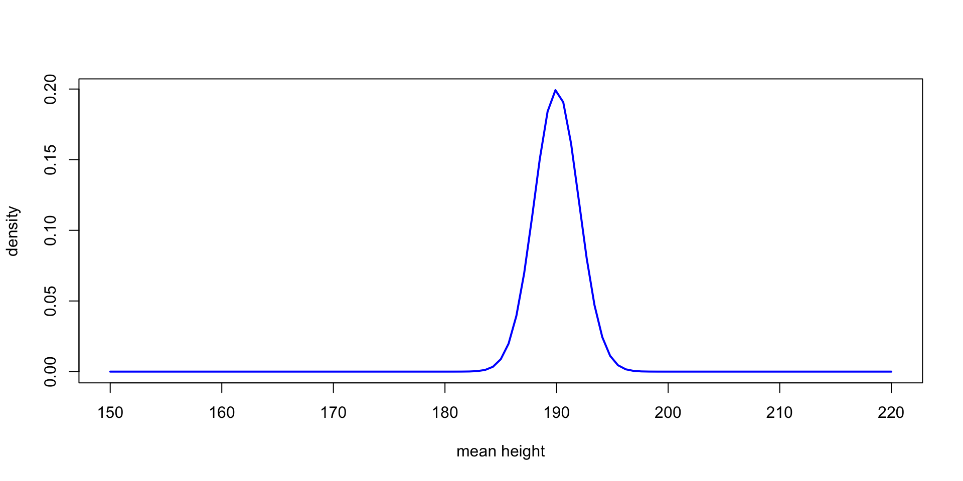
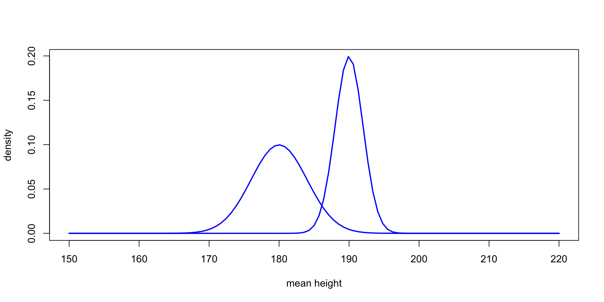
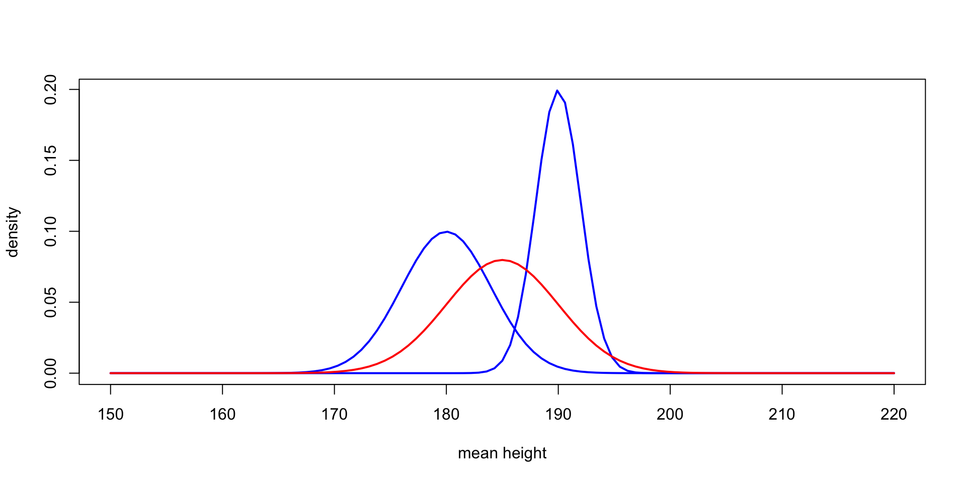
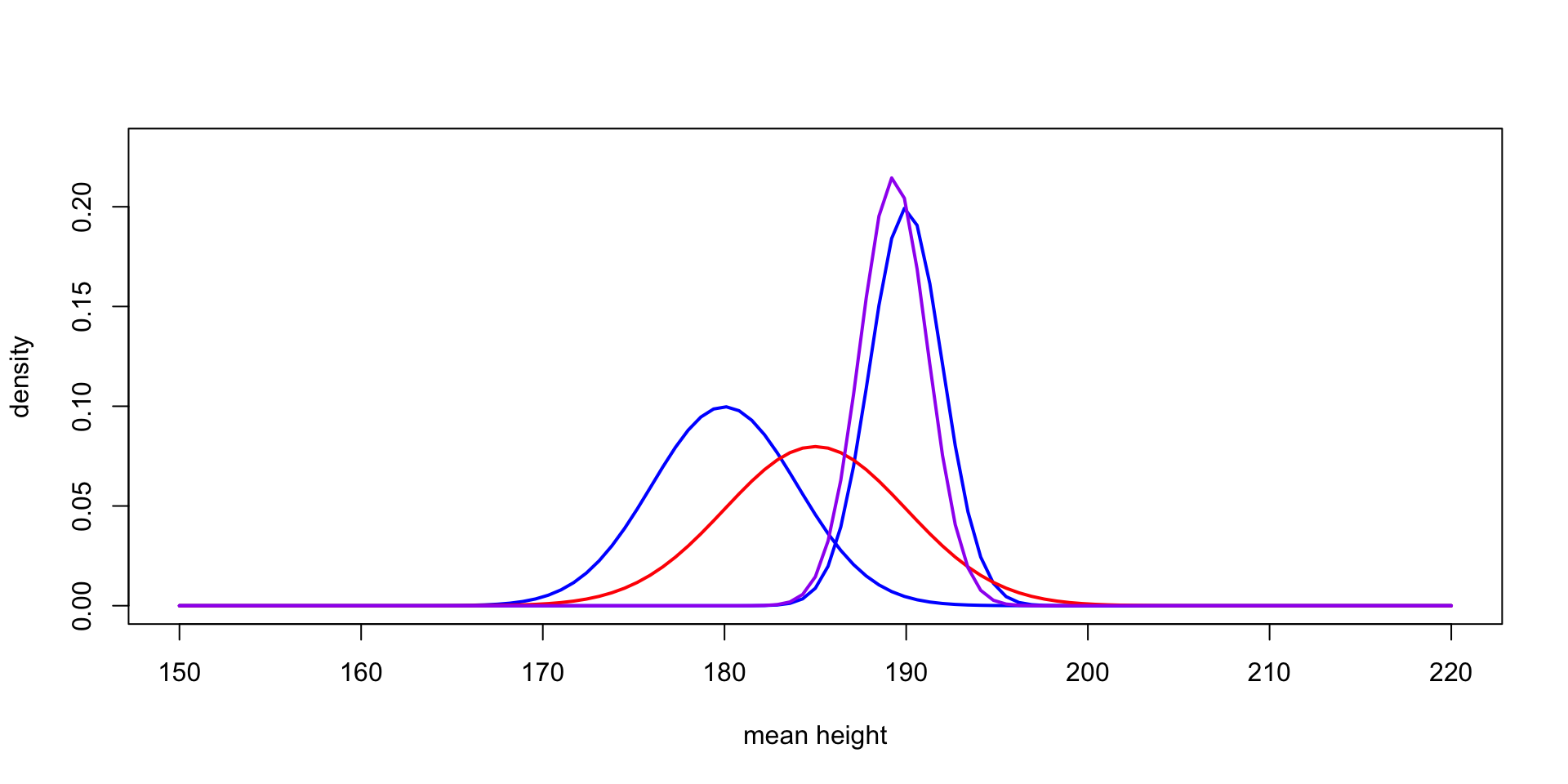
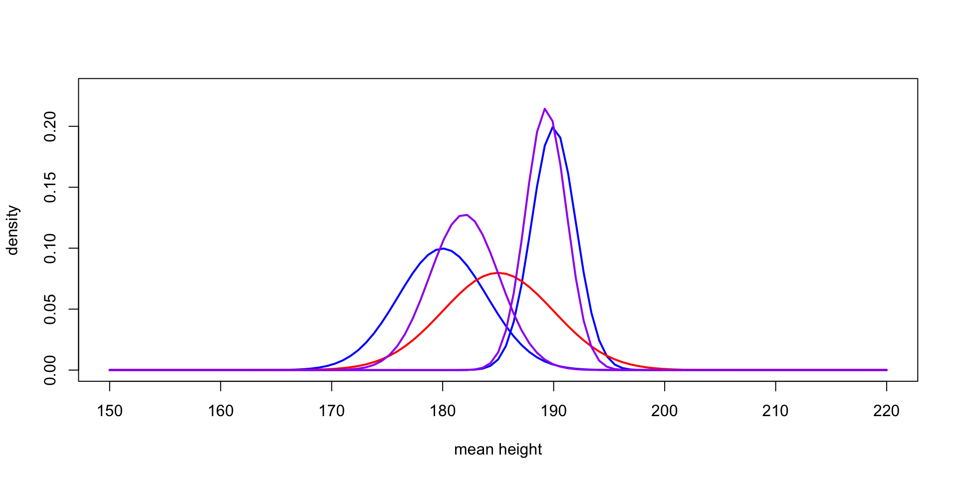
Walking through setting the prior
Exchangeability
Exchangeability is a critical concept to understand when discussing Bayesian models
Formally, when we say a sequence of random variables, \(Y_1, Y_2, Y_3, \dots, Y_n, \dots\) are exchangeable, the joint distribution of these variables does not change under any permuation of indices, denoted as \(Y_{\sigma(1)}, Y_{\sigma(2)}, Y_{\sigma(3)}, \dots, Y_{\sigma(n)}, \dots\)
Given a parametric density for \(Y_i\) dependent on \(\theta\), the assumption that the \(Y_i\) are conditionally indepdent given \(\theta\) and a prior for \(\theta\), then the marginal joint density for \(Y_i\) is exchangeable:
\[ p_{\mathbf{Y}}(y_1, y_2, \dots, y_n) = \int_{\Omega_\Theta} \prod_{i=1}^n p(y_i \mid \theta) p(\theta) d\theta \]
The idea goes the opposite direction as well: Given an infinite sequence of exchangeable random variables (this is true if, for every \(n\), the finite sequences are exchangeable), then there must exist a random variable \(\Theta\) such that the following holds \[ p_{\mathbf{Y}}(y_1, y_2, \dots, y_n) = \int_{\Omega_\Theta} \prod_{i=1}^n p(y_i \mid \theta) p(\theta) d\theta \]
Further, \(\lim_{n\to\infty}\frac{1}{n}\sum_{i=1}^n \to \Theta\)
Exchangeable sequences are positively correlated
Let \(Y_i, i = 1, 2, \dots\) be exchangeable
\[ \begin{aligned} \text{Cov}(Y_1, Y_2) & = \ExpA{\text{Cov}(Y_1, Y_2 \mid \theta)}{\Theta} + \text{Cov}_{\Theta}(\Exp{Y_1 \mid \theta}, \Exp{Y_2 \mid \theta}) \\ & \class{fragment}{{} = \text{Cov}_{\Theta}(\Exp{Y_1 \mid \theta}, \Exp{Y_2 \mid \theta})} \\ & \class{fragment}{{} = \VarA{\Exp{Y_1 \mid \theta}}{\Theta}} \\ & \class{fragment}{{} \geq 0} \end{aligned} \]
Normal models
Normal likelihoods are special for us statisticians because of the CLT (see § 5.5.3 in Casella and Berger (2024))
It is computationally convenient
pnormis implented in many many math libraries
It has nice analytical properties
Easy to bound normal densities and CDFs
Jointly normal RVs are conditionally normal
Convolved normals are normal
Normally distributed outcomes
Normal outcome \(y\) is real-valued
Mean \(\theta\) and variance \(\sigma^2\)
Density \[ p(\textcolor{red}{y} \mid \theta) = \frac{1}{\sqrt{2\pi}\sigma}\exp\lp-\frac{1}{2\sigma^2}(\textcolor{red}{y} - \theta)^2 \rp \]
\(\int_{-\infty}^{\infty} p(\textcolor{red}{y} \mid \theta) d\textcolor{red}{y} = 1\)
Normal likelihood
Likelihood for \(\theta\) (assuming \(\sigma^2\) is known!): \[ p(y \mid \textcolor{red}{\theta}) \propto \exp\lp-\frac{1}{2\sigma^2}(y - \textcolor{red}{\theta})^2 \rp \]
In the binomial example, we had \(p(y \mid \theta) \propto \theta^{y} (1 - \theta)^{n - y}\), so we could read off the conjugate prior,
Rearranging things in the normal likelihood will help us see the form of the conjugate prior
Normal likelihood in exponential family form
\[ \scriptsize \begin{aligned} p(y \mid \theta) & \propto \exp\lp-\frac{1}{2\sigma^2}(y - \theta)^2 \rp \\ & = \exp\lp-\frac{y^2}{2\sigma^2} + \frac{y}{\sigma^2} \theta -\frac{\theta^2}{2\sigma^2}\rp \\ & \propto \exp\lp\frac{\theta}{\sigma^2} y -\frac{\theta^2}{2\sigma^2}\rp \end{aligned} \]
Prior Form
- \[ \begin{aligned} p(\theta \mid \mu_0, \tau_0) & \propto \exp\lp \frac{\mu_0}{\tau_0^2} \theta - \frac{\theta^2}{2\tau_0^2}\rp \\ \end{aligned} \]
- Now we compute \(p(\theta \mid y, \mu_0, \tau_0) \propto p(y \mid \theta) p(\theta \mid \mu_0, \tau_0)\) \[ p(\theta \mid y, \mu_0, \tau_0) \propto \exp\lp\frac{\theta}{\sigma^2} y -\frac{\theta^2}{2\sigma^2}\rp \exp\lp \frac{\mu_0}{\tau_0^2} \theta - \frac{\theta^2}{2\tau_0^2}\rp \]
Working through the algebra
\[ \scriptsize \begin{aligned} & \exp\lp\theta\lp\frac{y}{\sigma^2} + \frac{\mu_0}{\tau_0^2}\rp -\frac{\theta^2}{2}\lp\frac{1}{\sigma^2} + \frac{1}{\tau_0^2} \rp\rp \\ & = \exp\lp\theta\lp\frac{\mu_1}{\tau_1^2}\rp -\frac{\theta^2}{2}\lp\frac{1}{\tau_1^2}\rp\rp \\ & \implies \end{aligned} \] \[ \scriptsize \begin{aligned} \frac{1}{\tau_1} & = \frac{1}{\sigma^2} + \frac{1}{\tau_0^2} && \frac{\mu_1}{\tau_1} = \frac{y}{\sigma^2} + \frac{\mu_0}{\tau_0^2} \\ \mu_1 & = \lp \frac{y}{\sigma^2} + \frac{\mu_0}{\tau_0^2}\rp \tau_1 && \mu_1 = \lp\frac{y}{\sigma^2} + \frac{\mu_0}{\tau_0^2}\rp / \lp \frac{1}{\sigma^2} + \frac{1}{\tau_0^2}\rp \end{aligned} \]
A tale of two likeihoods
Interpreting the parameters
- \[ \mu_1 = \mu_0 + (y - \mu_0) \frac{\tau_0^2}{\tau_0^2 + \sigma^2} \]
- vs. \[ \mu_1 = y - (y - \mu_0) \frac{\sigma^2}{\tau_0^2 + \sigma^2} \]
Posterior predictive distribution
We might want to make predictions for another observation
\[ p(\tilde{y} \mid y) = \int_{-\infty}^\infty p(\tilde{y} \mid \textcolor{red}{\theta}) p(\textcolor{red}{\theta} \mid y, \mu_0, \tau_0) d \textcolor{red}{\theta} \]
\[ \begin{aligned} & \int_{-\infty}^\infty p(\tilde{y} \mid \textcolor{red}{\theta}) p(\textcolor{red}{\theta} \mid y, \mu_0, \tau_0) d \textcolor{red}{\theta} \\ & = \int_{-\infty}^\infty \frac{1}{\sqrt{2\pi}\sigma}\exp(-\frac{1}{2\sigma^2}(y - \theta)^2)\frac{1}{\sqrt{2\pi}\tau_1}\exp(-\frac{1}{2\tau_1^2}(\theta_1 - \mu_1)^2) d \textcolor{red}{\theta} \end{aligned} \]
We can use the fact that \(\tilde{y} \mid \theta \sim \text{Normal}(\theta, \sigma^2)\) which is equal in distribution to \(Y = \theta + Z\) where \(Z \sim \text{Normal}(0, \sigma^2)\).
Marginally, \(Y \sim \text{Normal}(\mu_1, \tau_1^2 + \sigma^2)\)
Exponential families
The normal and binomial distributions are examples of a more general class of densities called exponential families
The exponential family distributions can be written in the following form
\[ p(y_i \mid \theta) = f(y_i) g(\theta)e^{\phi(\theta)^T u(y_i)} \]
With \(n\) iid observations, calling \(t(y) = \sum_{i=1}^n u(y_i)\) the joint density is \[ p(y \mid \theta) = \lp \prod_{i=1}^n f(y_i)\rp g(\theta)^n \exp \lp \phi(\theta)^T t(y)\rp \]
We can write the density as \[ p(y\mid \theta) \propto g(\theta)^n \exp \lp \phi(\theta)^T t(y)\rp \]
This shows that \(t(y)\) is sufficient for \(\theta\)
Conjugate priors in exponential families
When \[ p(y\mid \theta) \propto g(\theta)^n \exp \lp \phi(\theta)^T t(y)\rp \]
Specifying \(p(\theta) \propto g(\theta)^\eta \exp\lp \phi(\theta)^T \nu \rp\) yields the posterior:
\[ p(\theta \mid y) \propto g(\theta)^{n + \eta} \exp \lp\phi(\theta)^T(t(y) + \nu) \rp \]
Back to the normal again
With \(n\) observations, we know that \(\bar{y}\) is sufficient for \(\mu\) when \(y \sim \text{Normal}(\mu, \sigma^2)\)
We know \(\bar{y} \sim \text{Normal}(\mu, \frac{\sigma^2}{n})\), so we can just use our earlier results to get the posterior \(\mu_n\) and \(\tau_n\) parameters
\[ \scriptsize \begin{aligned} \frac{1}{\tau_n} & = \frac{n}{\sigma^2} + \frac{1}{\tau_0^2} \\ \mu_n & = \lp y \frac{n}{\sigma^2} + \frac{\mu_0}{\tau_0^2}\rp / \lp \frac{n}{\sigma^2} + \frac{1}{\tau_0^2}\rp \end{aligned} \]
As \(n\to\infty\) we get $_n \(\bar{y}\) and \(\tau^2_n \to \frac{\sigma^2}{n}\)
This shows that the posterior for \(\theta\) converges to a normal distribution with mean \(\bar{y}\) and \(\frac{\sigma^2}{n}\)
We get the same convergence in distribution if \(\tau_0 \to \infty\)
Models for count data
When we have \(y_i \in \{0\} \cup \Z^+\), we’ll need to use something other than a normal
One common model is \(y_i \sim \text{Poisson}(\theta)\) \[ p(y_i \mid \theta) = \frac{e^{-\theta} \theta^y_i}{y_i!} \]
Rewrite this in exponential family form: \[ e^{-\theta} e^{\log(\theta) y} \]
Suggests a prior of the form \[ \begin{aligned} p(\theta) & \propto e^{-\theta \eta} e^{\log(\theta) \nu} \\ & \propto \theta^\nu e^{-\theta \eta} \end{aligned} \]
This is a Gamma distribution, or \(p(\theta) = \frac{\beta^\alpha}{\Gamma(\alpha)} \theta^{\alpha - 1} e^{-\beta \theta}\)
Multiple observations
With \(n\) iid observations the joint density for \(y\) is \[ \begin{aligned} p(y \mid \theta) & \propto e^{-n\theta} e^{\log(\theta) \sum_{i=1}^n y_i} \\ & \propto e^{-n\theta} \theta^{\sum_{i=1}^n y_i} \\ & \propto e^{-n\theta} \theta^{t(y)} \end{aligned} \]
With a prior \(p(\theta) \propto \theta^{\alpha - 1} e^{-\beta \theta}\) we get
Posterior \[ p(\theta \mid y) \propto e^{-\theta(n + \beta)} \theta^{t(y) + \alpha} \]
Or \(\theta \mid y \sim \text{Gamma}(\alpha + t(y), \beta + n)\)
Deriving the prior/posterior predictive distribution
\[ \begin{aligned} & \frac{\beta^\alpha}{y!\Gamma(\alpha)} \int_0^\infty e^{-\theta} \theta^y \theta^{\alpha - 1} e^{-\beta \theta} d\theta \\ & \class{fragment}{{} = \frac{\beta^\alpha}{y!\Gamma(\alpha)} \int_0^\infty \theta^{y + \alpha - 1} e^{-\theta(\beta + 1)} d\theta} \\ & \class{fragment}{{} = \frac{\beta^\alpha}{y!\Gamma(\alpha)}\frac{\Gamma(\alpha + y)}{(\beta + 1)^{\alpha + y}}} \\ & \class{fragment}{{}= \frac{\Gamma(\alpha + y)}{y!\Gamma(\alpha)}\lp\frac{\beta}{\beta + 1}\rp^\alpha \lp\frac{1}{\beta + 1}\rp^y} \end{aligned} \]
Negative binomial distribution
Last slide we derived negative-binomial distribution with parameters \(\alpha\) and \(\beta\)
How might we get the mean and variance of this distribution?
We can get it by \(y \mid \theta \sim \text{Poisson}(\theta)\) and \(\theta \sim \text{Gamma}(\alpha, \beta)\).
\(\Exp{y} = \ExpA{\Exp{y \mid \theta}}{\theta}\)
- \(\Var{y} = \ExpA{\Var{y \mid \theta}}{\theta} + \VarA{\Exp{y \mid \theta}}{\theta}\)
- Can be useful to reparameterize in terms of mean and dispersion parameter
Poisson with rate/exposure parameterization
Many times it is useful to specify the model for count data \(y_i\) as conditional on an unknown rate and a known exposure term \(x_i\) \[ y_i \sim \text{Poisson}(x_i \theta) \]
We can see that this model is no longer exchangeable in \(y_i\), but is exchangeable in \((y_i, x_i)\)
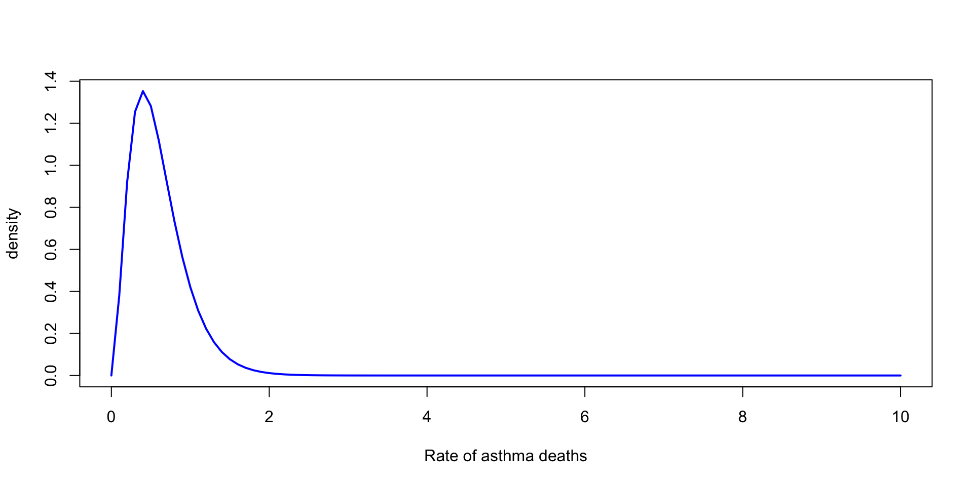
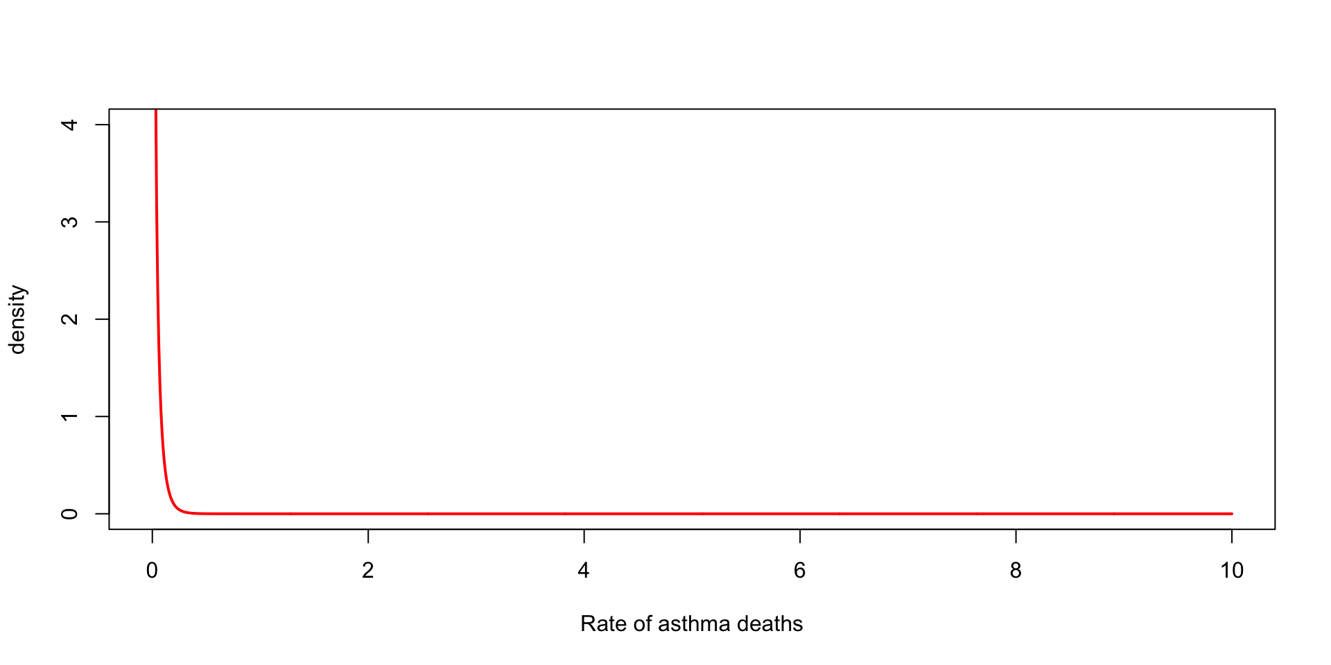
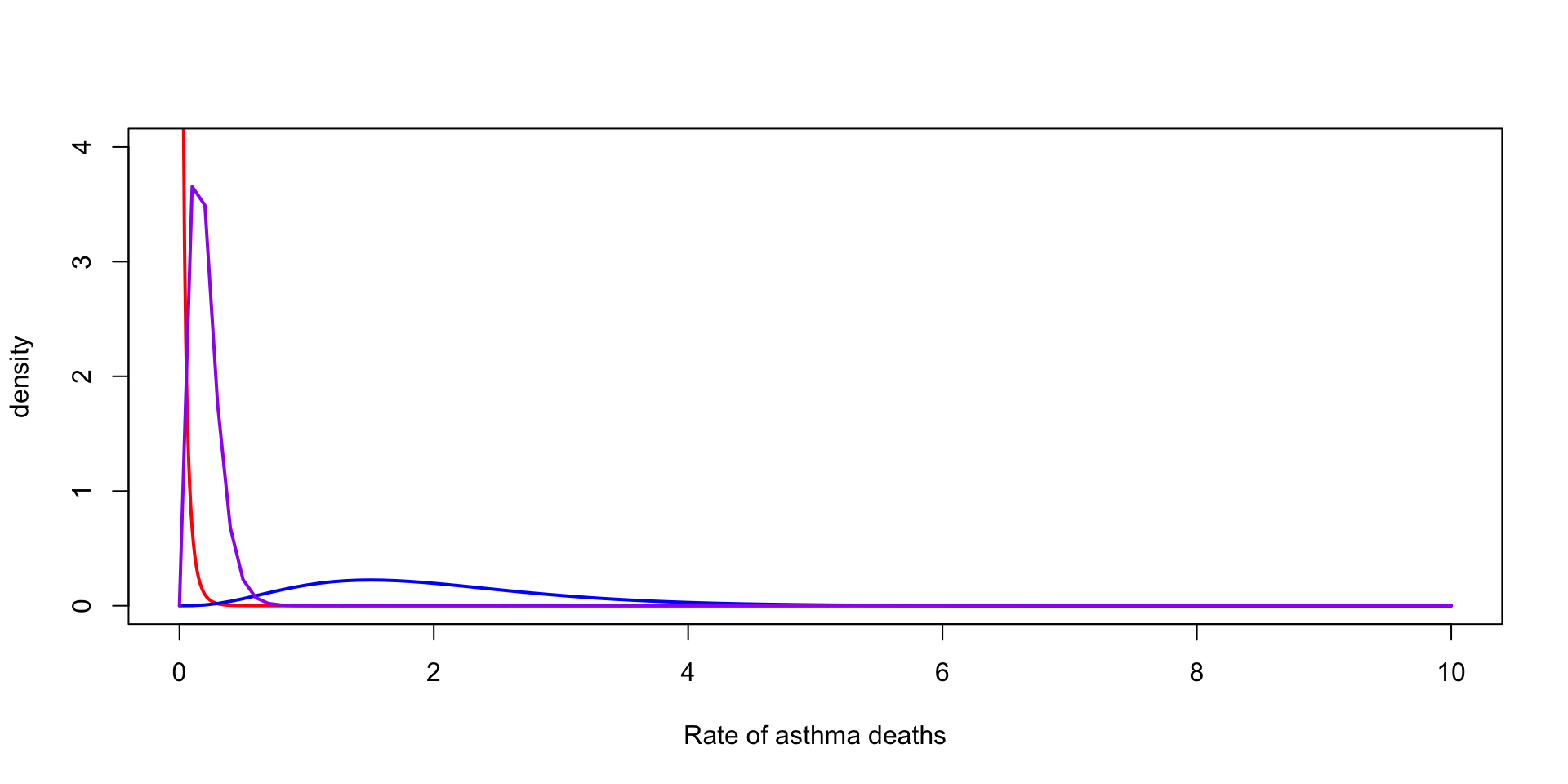
Often useful in epidemiological settings, where we want to model the rate of, say, cancer cases per person per year
Suppose we observe \(3\) death from asthma over one year for a city of \(200,000\)
We want to model the rate of deaths from asthma per \(100{,}000\)
\(y_1 \sim \text{Poisson}(2\, \theta) \rightarrow \theta \mid y_1 \sim \text{Gamma}(\alpha + 3, \beta + 2)\)
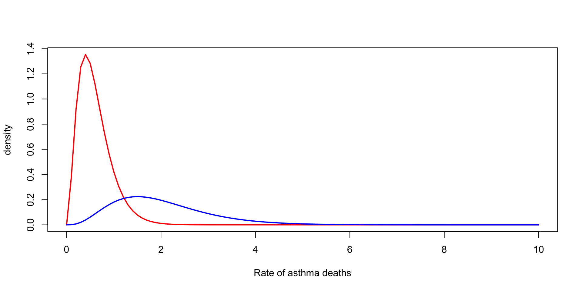
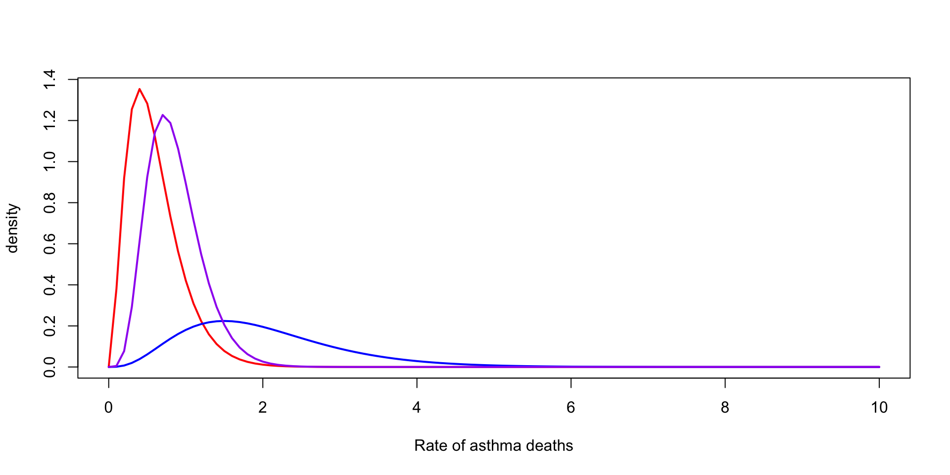
Scale of the prior
Normal with known mean
Though not typical of real-world scenarios, under \(y_i \mid \theta, \sigma^2 \sim \text{Normal}(\theta, \sigma^2)\) we can derive the posterior for \(\sigma^2\) under the assumption that \(\theta\) is known
The likelihood corresponding the joint distribution of \(Y_1, Y_2, \dots, Y_n\) is \[ p(y \mid \sigma^2, \theta) = \prod_{i=1}^n \frac{1}{\sqrt{2\pi\sigma^2}} \exp \lp -\frac{1}{2\sigma^2} (y_i - \theta)^2 \rp \]
Simplifying and dropping constants \[ p(y \mid \sigma^2, \theta) \propto (\sigma^2)^{-n/2}\exp \lp -\frac{1}{2\sigma^2} \sum_{i=1}^n (y_i - \theta)^2 \rp \]
Let’s represent \(\sum_{i=1}^n (y_i - \theta)^2\) as \(n v\), so we rewrite this as: \[ p(y \mid \sigma^2, \theta) \propto (\sigma^2)^{-n/2}\exp \lp -\frac{n}{2\sigma^2} v \rp \]
The conjugate prior here is called the inverse gamma, \[ p(\sigma^2 \mid \alpha, \beta) = \frac{\beta^\alpha}{\Gamma(\alpha)} (\sigma^2)^{-(\alpha+1)} e^{-\beta/\sigma^2} \]
The posterior gives \[ p(\sigma^2 \mid y, \theta, \alpha, \beta) \propto (\sigma^2)^{-(n/2 + \alpha+1)} \exp \lp -(\frac{n}{2} v + \beta)/\sigma^2\rp \]
References
Casella, George, and Roger Berger. 2024. Statistical Inference. Chapman; Hall/CRC.