[1] 1[1] 1.145624e-42\(\Exp{\theta} = \sum_{s=1}^S \theta^{(s)} w^{(s)}\)
More sophisticated methods are available in R using the integrate function
Evaluations increase exponentially as the dimension of the space increases \(c^d\)
A significant hurdle in grid methods is that you have to define the grid before you know where the mass of the probability distribution
Approximate cost: Suppose we have \(50\) points in each dimension and \(10\) dimensions, this would require \(50^{10} \approx 1e17\) evaluations
Even with a fast computer, this could take years to evaluate
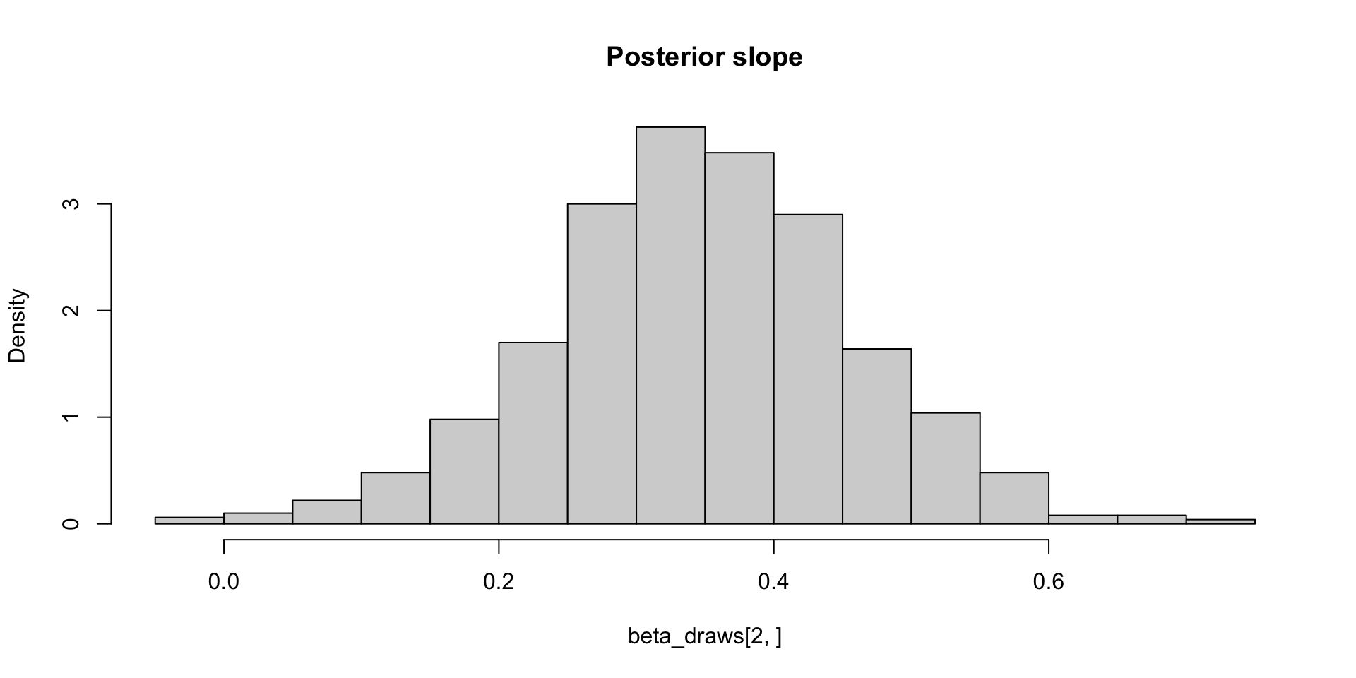
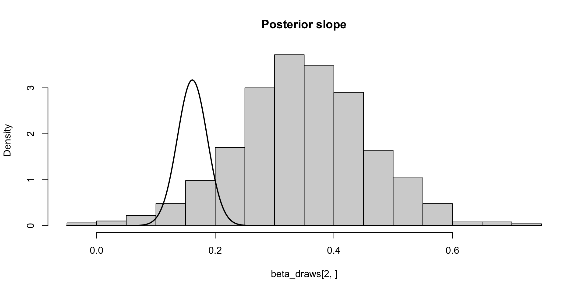
\[ \sigma_\theta \approx 0.12 \implies \text{MCSE}(\hat{\mathbb{E}}[\beta_2 \mid y]) \approx 0.12 / 10 \]

\[ \sigma_\theta \approx 0.12 \implies \text{MCSE}(\hat{\mathbb{E}}[\beta_2 \mid y]) \approx 0.12 / 10 \\ P(\Exp{\beta_2 \mid y} \in (0.33, 0.38)) \approx 0.95 \]

\[ \sigma_\theta \approx 0.12 \implies \text{MCSE}(\hat{\mathbb{E}}[\beta_2 \mid y]) \approx 0.12 / \sqrt{1000} \\ P(\Exp{\beta_2 \mid y} \in (0.35, 0.36)) \approx 0.95 \]
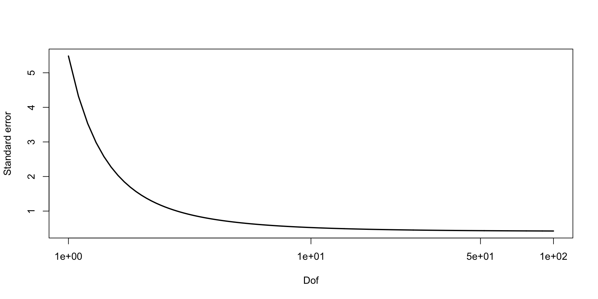
\[\hat{F}^{-1}(\alpha) \overset{\text{d}}{\to} N(a, \alpha (1 - \alpha) / f(a)^2 S)\]
\[ \text{MCSE}(\hat{F}_{\beta_2 \mid y}^{-1}(0.05)) \approx \sqrt{0.05 \times 0.95} / 10 f(q) \approx 0.03 \\ P(F_{\beta_2 \mid y}^{-1}(0.05) \in (0.11, 0.21)) \approx 0.95 \]

\[ \text{MCSE}(\hat{F}_{\beta_2 \mid y}^{-1}(0.05)) \approx \sqrt{0.05 \times 0.95 / 1000 f(q)} \approx 0.01 \\ P(F_{\beta_2 \mid y}^{-1}(0.05) \in (0.14, 0.18)) \approx 0.95 \]
\[ \text{MCSE}(\hat{F}_{\beta_2 \mid y}^{-1}(0.05)) \approx \sqrt{0.01 \times 0.99} / 10 f(q) \approx 0.04\\ P(F_{\beta_2 \mid y}^{-1}(0.01) \in (-0.01, 0.15)) \approx 0.95 \]
\[ \text{MCSE}(\hat{F}_{\beta_2 \mid y}^{-1}(0.05)) \approx \sqrt{0.01 \times 0.99 / 1000f(q)} \approx 0.02 \\ P(F_{\beta_2 \mid y}^{-1}(0.01) \in (0.03, 0.11)) \approx 0.95 \]
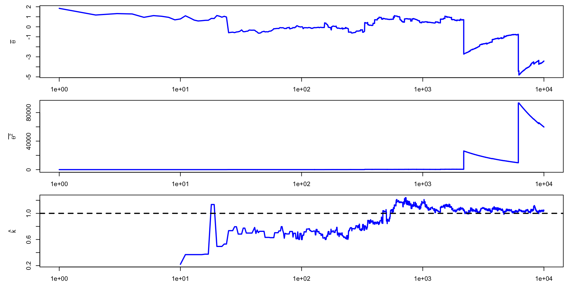
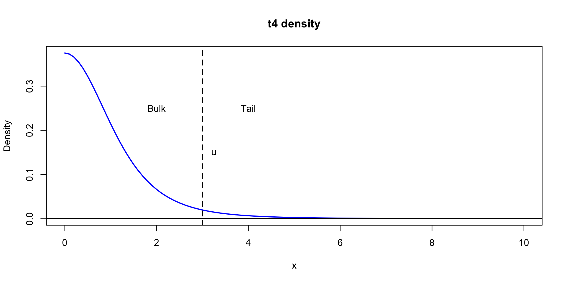
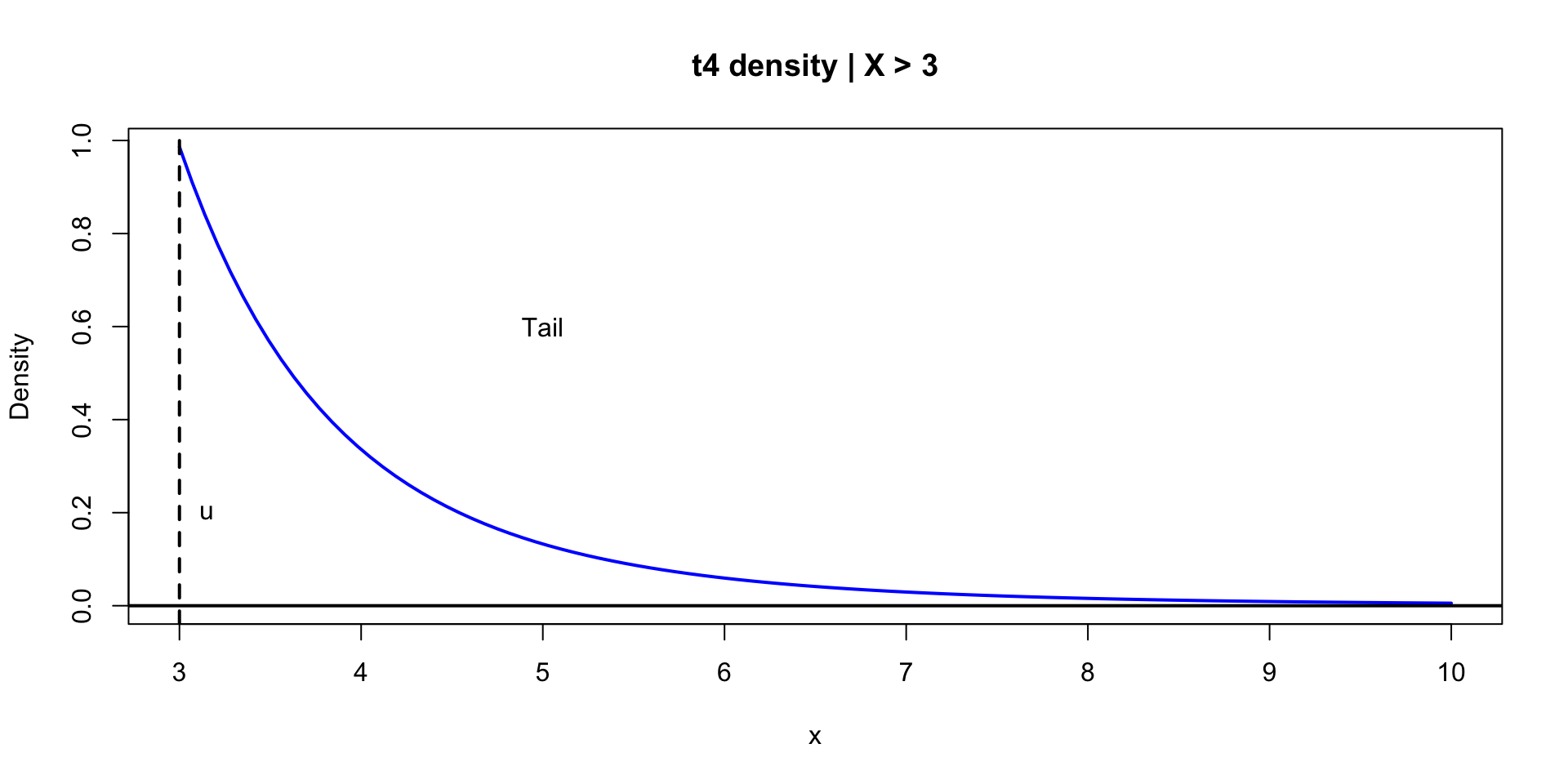
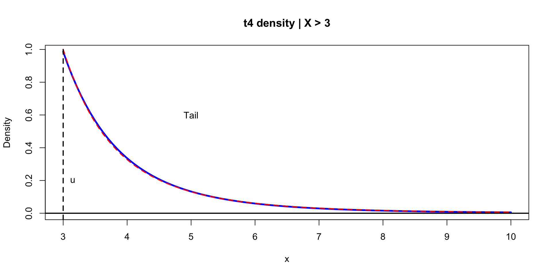
\[ p(y \mid u, \sigma, k) = \begin{cases} \frac{1}{\sigma}(1 + k \lp \frac{y - u}{\sigma} \rp)^{-(1 + 1/k)}, & k \neq 0 \\ \frac{1}{\sigma}\exp\lp \frac{y - u}{\sigma} \rp), & k = 0 \end{cases} \]
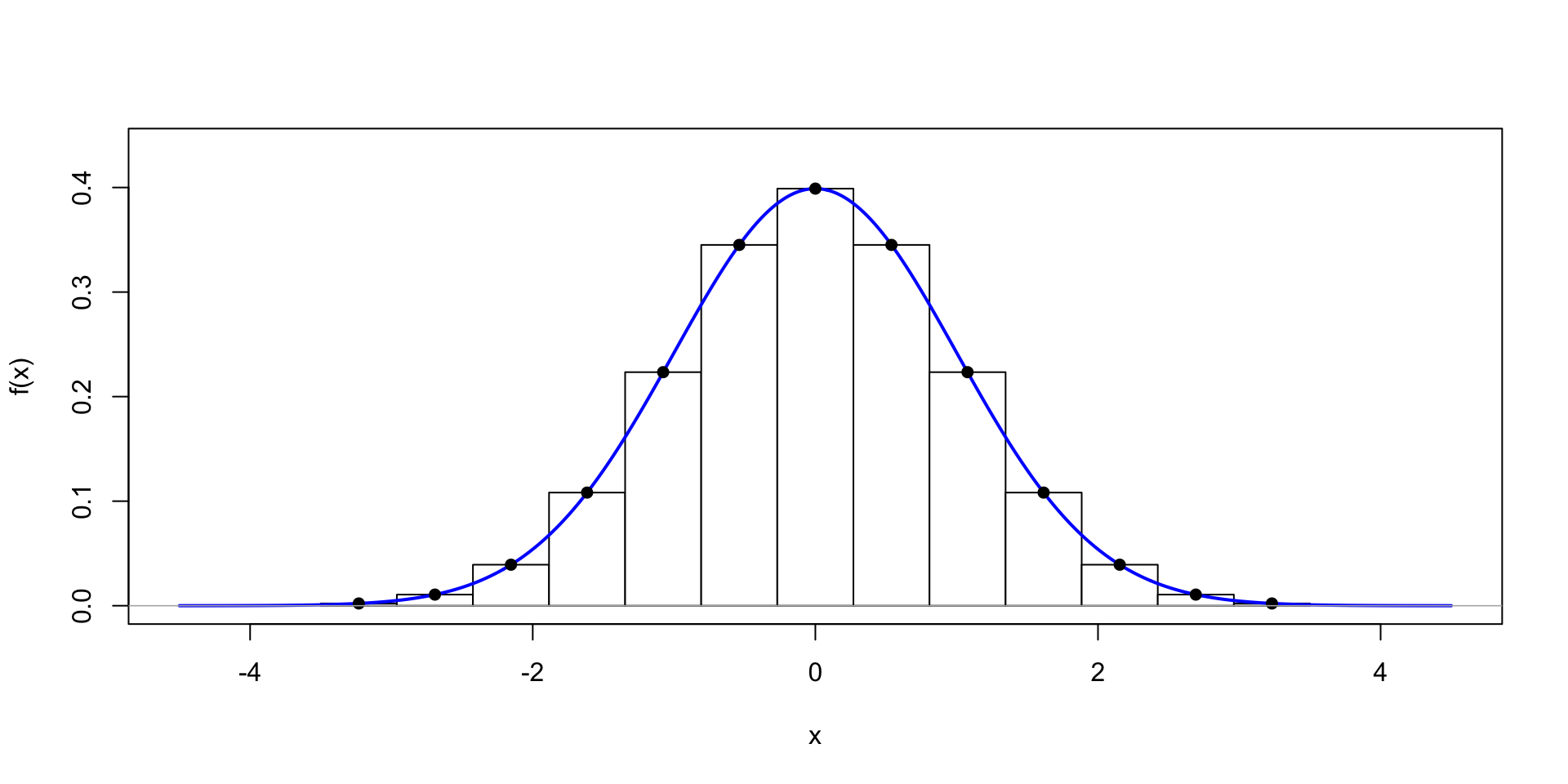
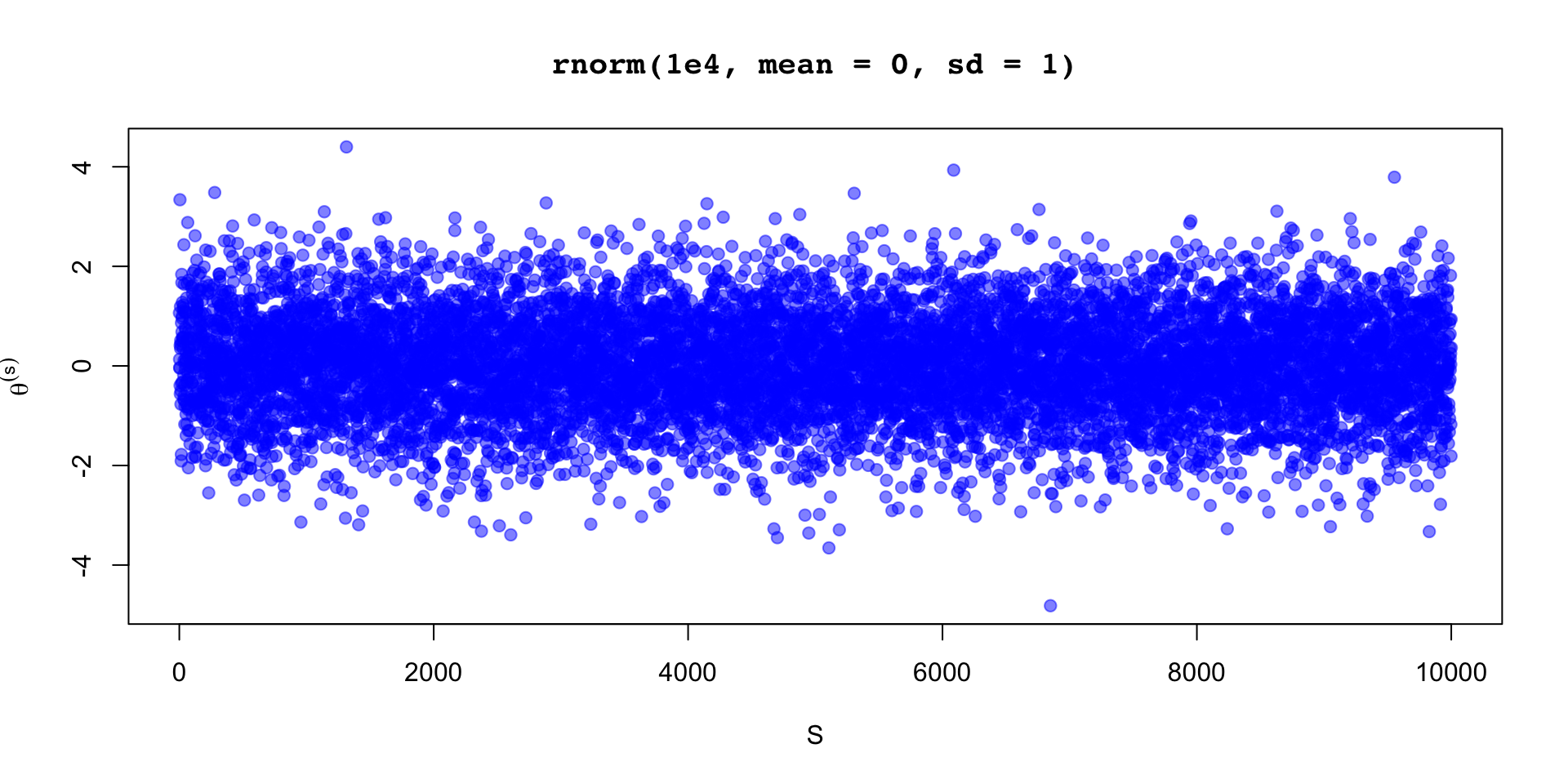
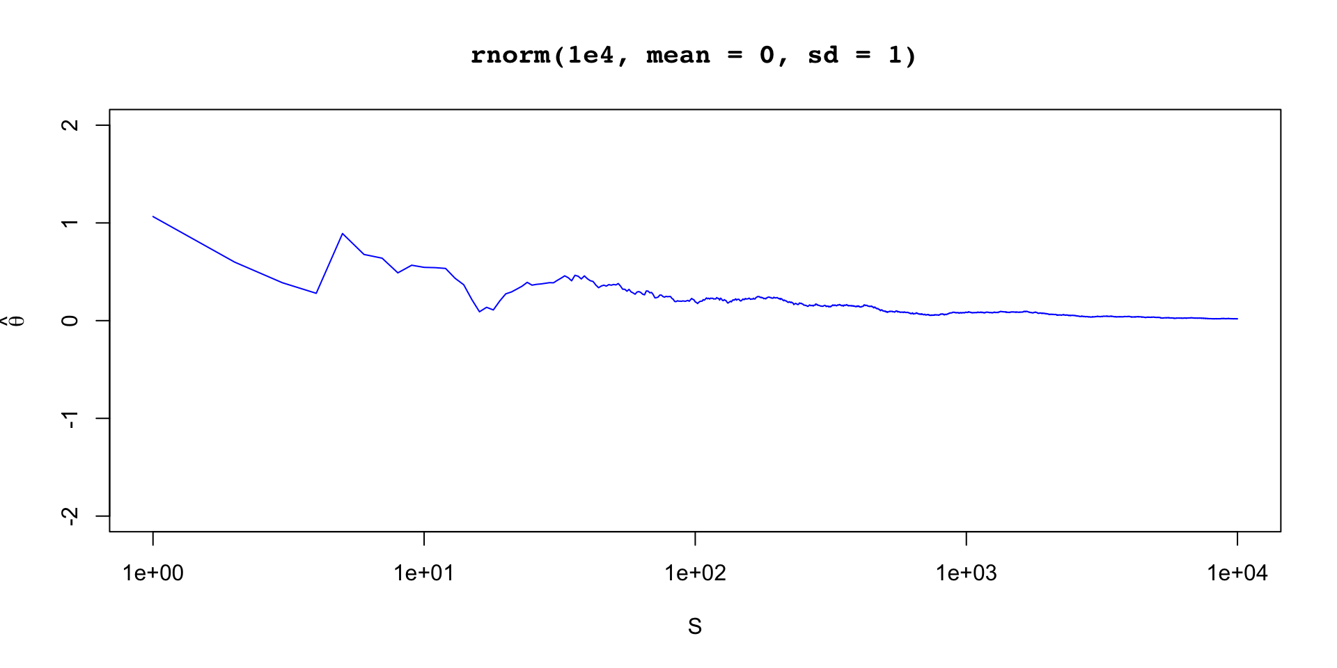
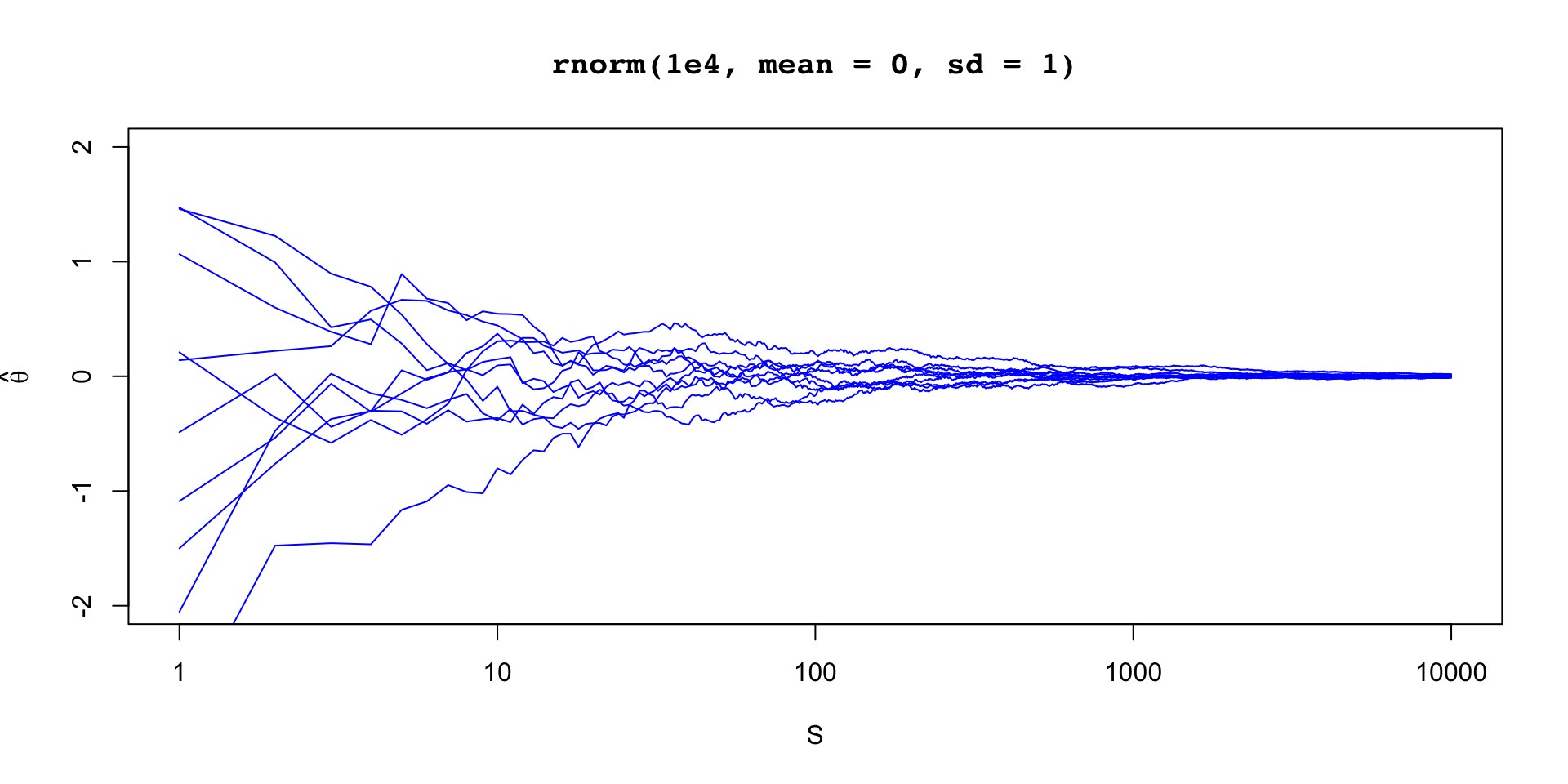
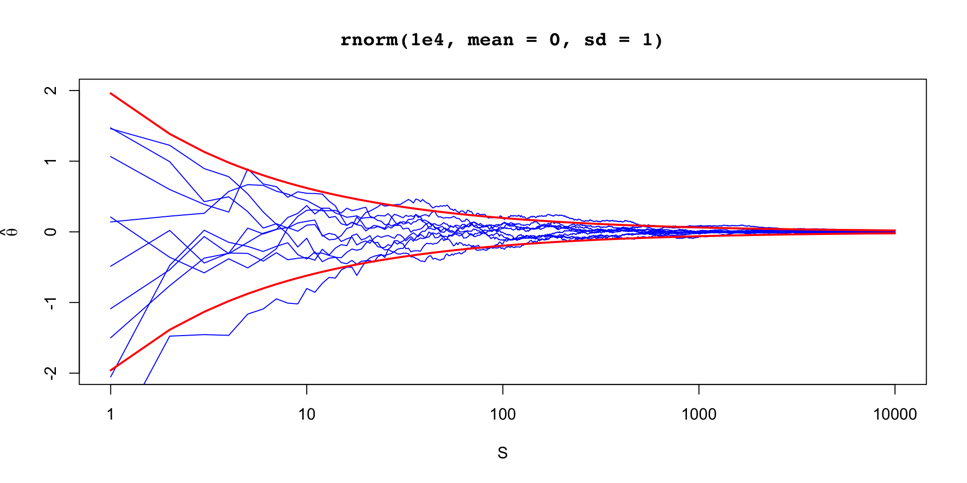
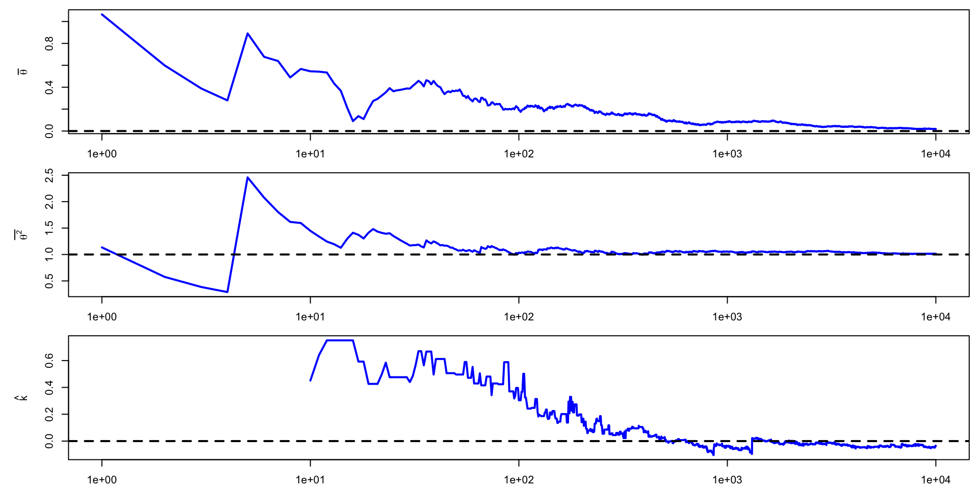
\(\theta \sim \text{Normal}(0,1)\)
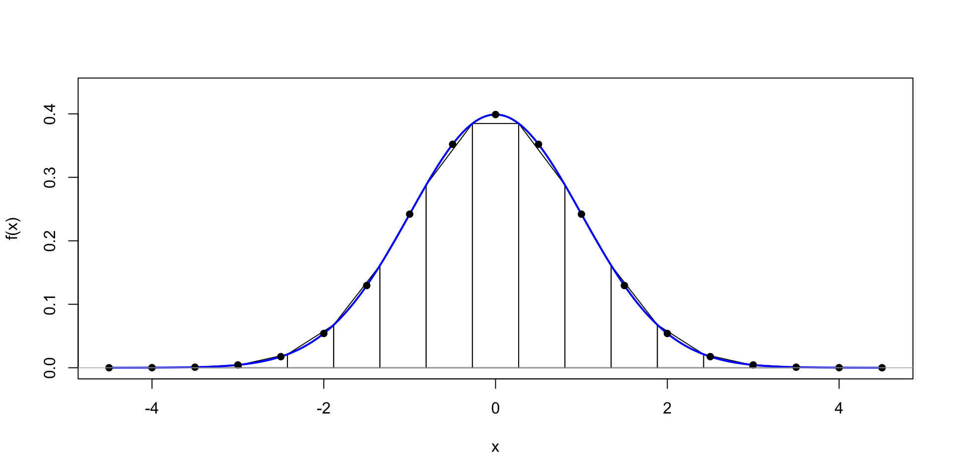
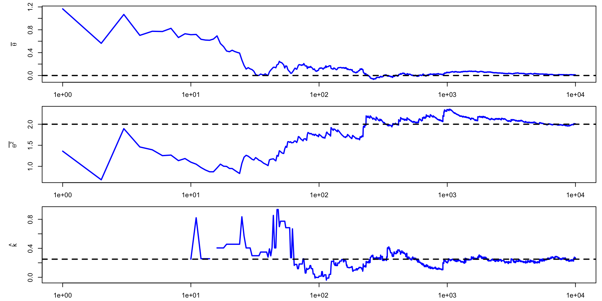
\(\theta \sim \text{t}(4, 0,1)\)
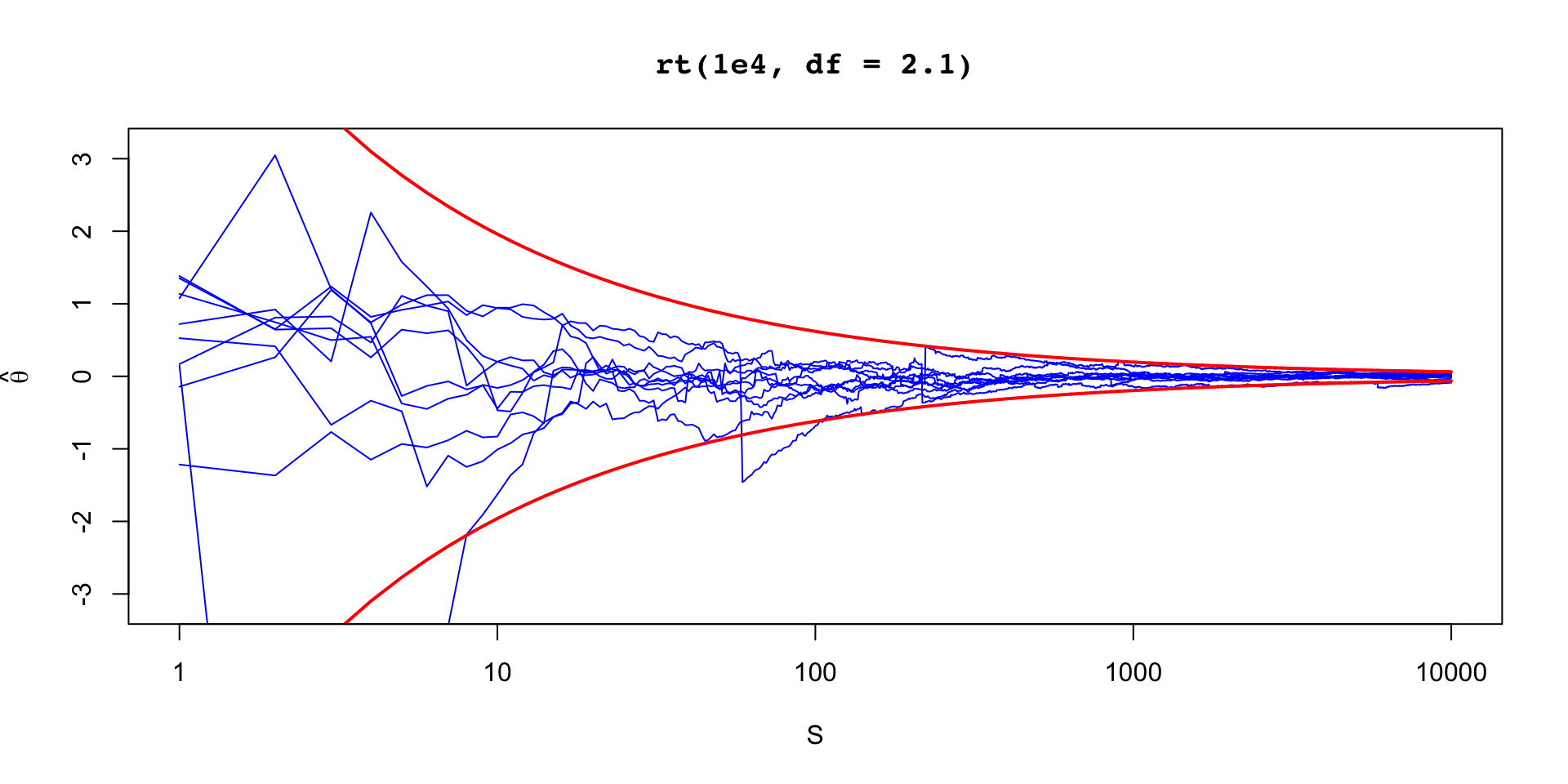
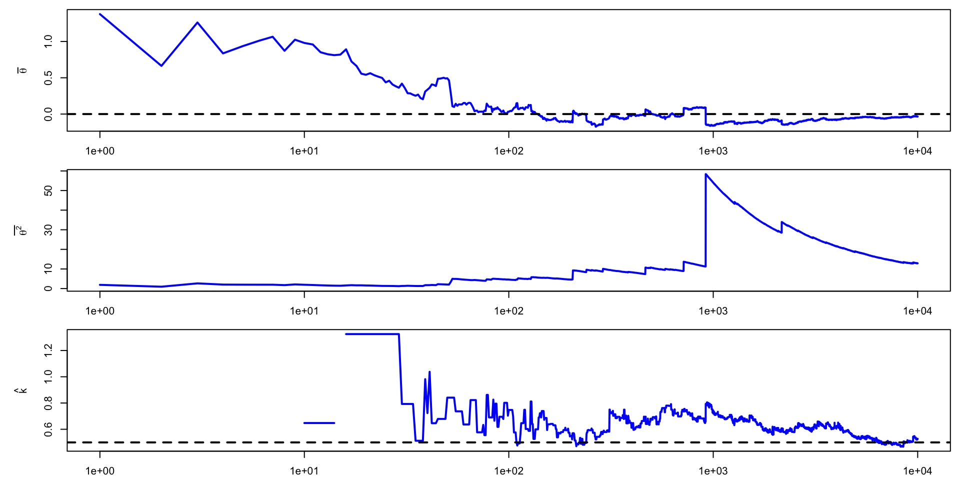
\(\theta \sim \text{t}(2, 0,1)\)
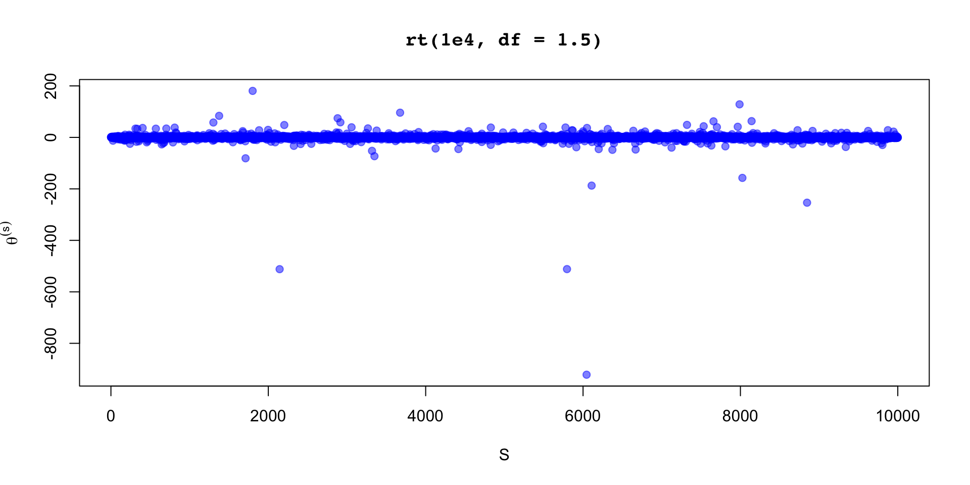
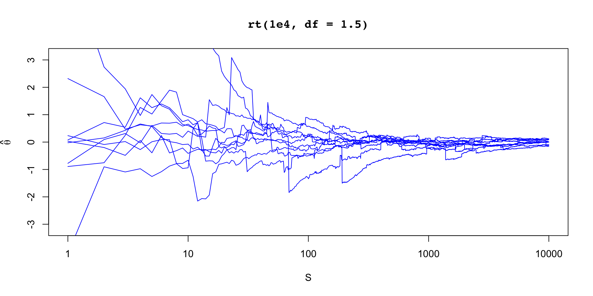
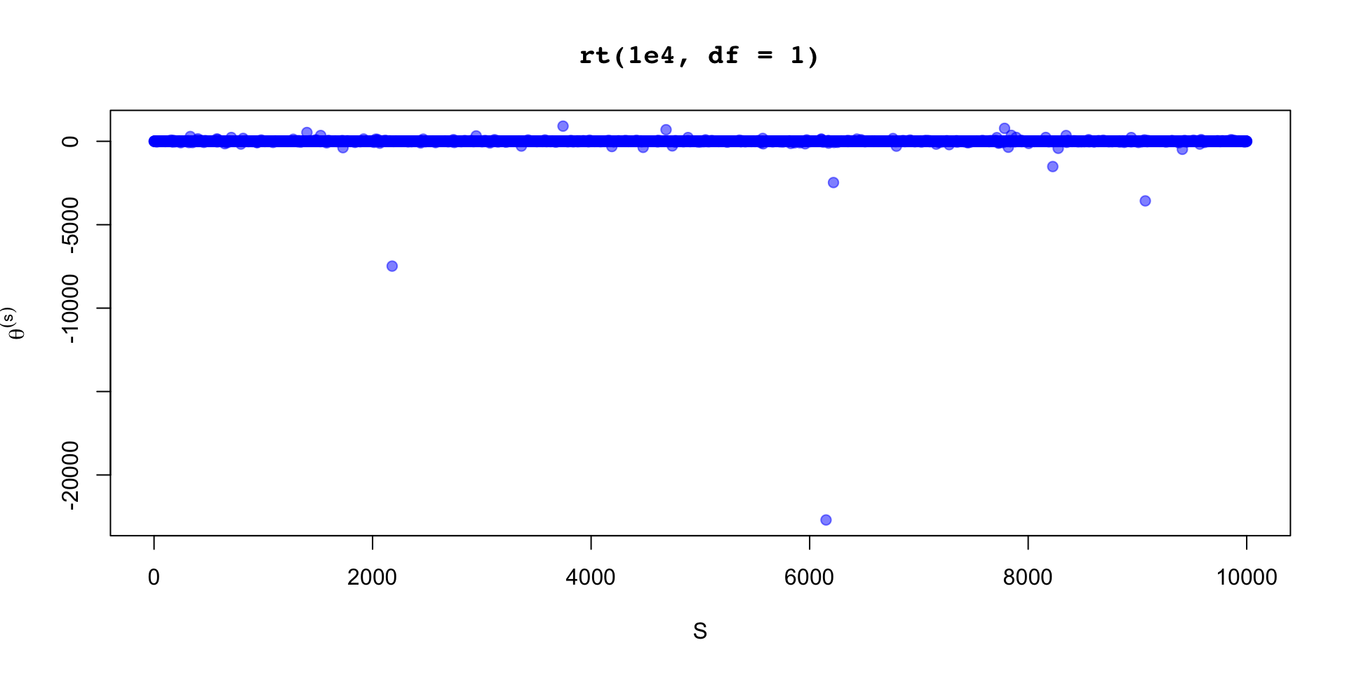
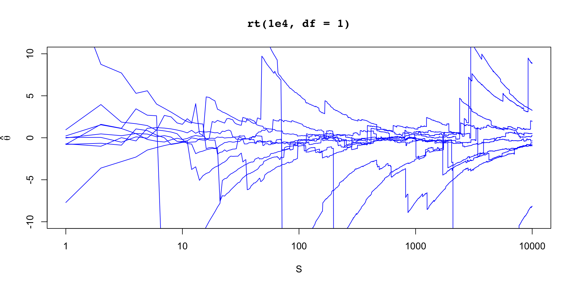
\(\theta \sim \text{t}(1, 0,1)\)