ST 559: Introduction
“Classical” approach to statistics
Data \(Y\) is assumed to arise from a model \(f_Y(y \mid \theta)\)
Choose a class of estimators (unbiased, maximum likelihood, least squares, etc.)
Infer \(\hat{\theta}\) from \(Y\)
Calculate the sampling distribution \(\hat{\theta}\) assuming repeated draws from \(f_Y(y \mid \theta)\).
Issue 1: Consequences (losses)
On its face, classical statistics seems fine
However, as L.J. Savage puts it in Savage (1972):
[…] the problems of statistics were almost always thought of as problems of deciding what to say rather than what to do
Namely, the end use (and end user) of an estimate isn’t considered
Consider two scenarios:
\(\theta\) represents the expected proportion of NYTimes app users who click on a banner ad (what is the consequence of underestimation for the NYT?)
\(\theta\) represents the expected proportion of cancer patients for whom a new treatment leads to remission (what is the consequence of underestimation for the researchers?)
Solutions to problem 1: Decision theory and loss functions
You’ve already seen some decision theory in ST 562
Let the set of actions one can take be \(\mathcal{A}\) and let the true state of nature be \(\theta\).
A loss function for a single action, \(a\), is \(L(a, \theta)\), which maps an action (or a decision) and the state of nature to a number representing the cost of the action
Examples: squared error: \(L(a,\theta) = (a - \theta)^2\), absolute error: \(L(a,\theta) = \abs{a - \theta}\)
Solutions to problem 1: More involved loss functions
Asymmetric loss:
- \[ L(a,\theta) = \begin{cases} 10(a - \theta)^2 & a < \theta \\ (a - \theta)^2 & a \geq \theta \end{cases} \]
Linear loss under discrete actions \(a \in \{1, 2\}\)
- \[ L(a, \theta) = \begin{cases} K_1 + k_1 \theta & a = 1 \\ K_2 + k_2 \theta & a = 2 \end{cases} \]
Issue 2: Importance of context in statistics
A (modified) example from L.J. Savage: Consider the following experiments in which we are trying to infer \(\theta\), the probability that a person will answer a question correctly:
A self-described coffee expert claims to be able to determine whether his iced latte was made with milk poured into the cup prior to the espresso shot or if the espresso shot went in first followed by the milk. In a randomized experiment, he correctly identifies the order 10 out of 10 times
An internationally renowned beer expert claims to be able to distinguish West Coast IPAs from New England IPAs. She correctly identifies the beers in a randomized study 10 out 10 times.
You are celebrating an OSU win over UO baseball at Squirrel’s when you meet a dejected Duck fan who swears he is clairvoyant and can predict the outcome of a fair coin flip. He correctly predicts 10 out of 10 flips.
Issue 2: Importance of context in statistics
Berger (2013) notes: each example in the previous slide would lead to an MLE for \(\theta = 1\), and a classical hypothesis test would yield a p-value of \(2^{-10}\) under the null \(\theta = 1/2\).
However, the weight we would give the evidence in each example would differ (How would we weigh the different examples?)
Bayesian inference
Bayesian inference is a way of weighing evidence from the likelihood against a prior distribution
A Bayesian probability model has two pieces
Likelihood: \(f_Y(y \mid \theta)\), or the sampling distribution for the data
Prior: \(p(\theta)\), which measures the beliefs about \(\theta\) prior to observing data \(Y\)
Bayesian inference cont’d
- Bayesian inference uses Bayes’ rule to update the prior to a posterior:
\[ p(\theta \mid y) = \frac{f_Y(y \mid \theta) p(\theta)}{\int_{\Theta} f_Y(y \mid \theta) p(\theta) d\theta} \]
Sources of uncertainty
“Aleatoric” uncertainty means stochastic uncertainty; this is the uncertainty that frequentist statistics considers
Coin flips, measurement error, sampling uncertainty
For a given dataset, there is no uncertainty in frequentism
“Epistemic” uncertainty is uncertainty due to lack of knowledge: Bayesian inference adds epistemic uncertainty
The prior and the posterior track epistemic uncertainty
This is what allows us to make probability statements conditional on a given dataset
Different observers can have different knowledge of a problem
Example: Drawing colored poker chips from a bag
Probability of red \(\theta = \frac{\textcolor{red}{\text{\#red}}}{\textcolor{red}{\text{\#red}} + \textcolor{orange}{\text{\#orange}}}\)
\(Y_i\) is the color of a draw with replacement from the bag, \(p(Y_i = \textcolor{red}{\text{red}} \mid \theta)\): aleatoric uncertainty
\(p(\theta)\): epistemic uncertainty
Picking chips from the bag will change our uncertainty about the proportion
\(p(\theta \mid \textcolor{red}{\text{red}}, \textcolor{orange}{\text{orange}}, \textcolor{orange}{\text{orange}}, \textcolor{red}{\text{red}}, \dots) = ?\)
Use Bayes rule: \[ p(\theta \mid y) = \frac{f_Y(y \mid \theta) p(\theta)}{\int_{\Theta} f_Y(y \mid \theta) p(\theta) d\theta} \]
Fundamental understandings of probability
Frequentist probability is, as the name implies, defined by long-run frequencies of outcomes
- This seems like a good mathematical model for simple outcomes like dice throws, or poker hands, but doesn’t make as much sense for modeling outcomes like the winner of the Michigan/Arizona Basketball game on Saturday
Bayesian probability, in contrast, measures degrees of belief, and can be constructed from a coherent betting strategy on the outcomes of events
Frequentist vs. Bayesian uses of the loss function
The Bayesian approach to using the loss function is straightforward:
Given a posterior \(p(\theta \mid y)\), for each action \(a\) compute \(\rho(a) = \ExpA{L(a, \theta)}{\theta \mid y}\)
Pick the action that minimizes the expected loss: \(a^* = \argmin_a \rho(a)\)
The Frequentist approach to using the loss function is more involved
Frequentist use of the loss function
There is no epistemic uncertainty in frequentist inference, so we can’t compute \(\rho(a)\).
Instead we need a way to choose an \(a\) given a dataset, \(Y\), which we’ll denote \(\delta_k(y)\).
Then we compute risk, \(R(\delta_k, \theta) = \ExpA{L(\delta_k(Y), \theta)}{Y \mid \theta}\)
We can then rank decision rules \(\delta_m\) vs. \(\delta_k\) by comparing \(R(\delta_k, \theta)\) and \(R(\delta_j, \theta)\)
For instance, we can pick a decision rule by minimizing the maximum risk: \(\argmin_{k} \sup_{\theta} R(\delta_k, \theta)\)
Key differences
Bayesian model building is separate from a loss function
Frequentist model building is dependent on the loss function
Hurdle to Bayesian inference: Computation
Calculating integrals in the denominator is hard
\[ p(\theta \mid y) = \frac{f_Y(y \mid \theta) p(\theta)}{\int_{\Theta} f_Y(y \mid \theta) p(\theta) d\theta} \]
Directly approximating \[\int_{\Theta} f_Y(y \mid \theta) p(\theta) d\theta,\] is hard for reasons we’ll get into later in the course
Monte Carlo approximation of integrals
An alternative is to approximate functionals of the posterior:
\(\ExpA{f(\theta)}{\theta \mid y} = \int_{\Theta} f(\theta) p(\theta \mid y) d\theta\)
If we can draw \(\theta^{(s)}, s = 1, \dots, S\) from \(p(\theta \mid y)\), then \[\ExpA{f(\theta)}{\theta \mid y} \approx \frac{1}{S} \sum_{s=1}^S f(\theta^{(s)})\] by the WLLN
But how do we draw \(\theta^{(s)} \sim p(\theta \mid y)\)?
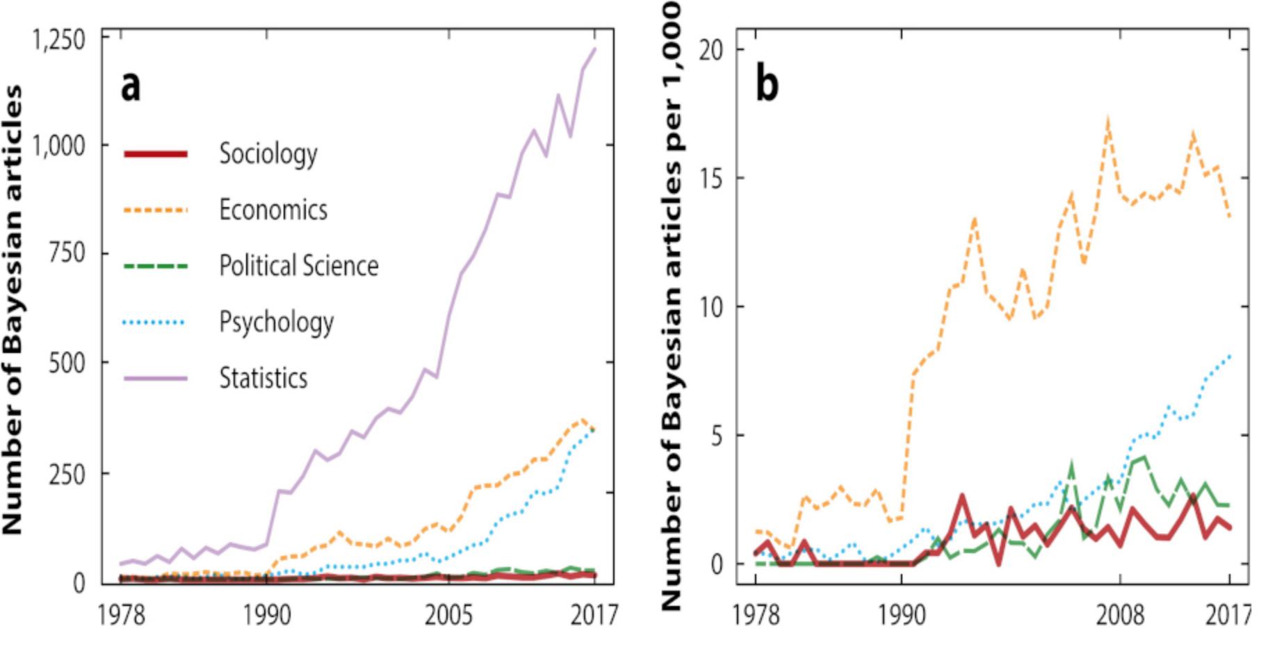
Bayesian Articles over Time
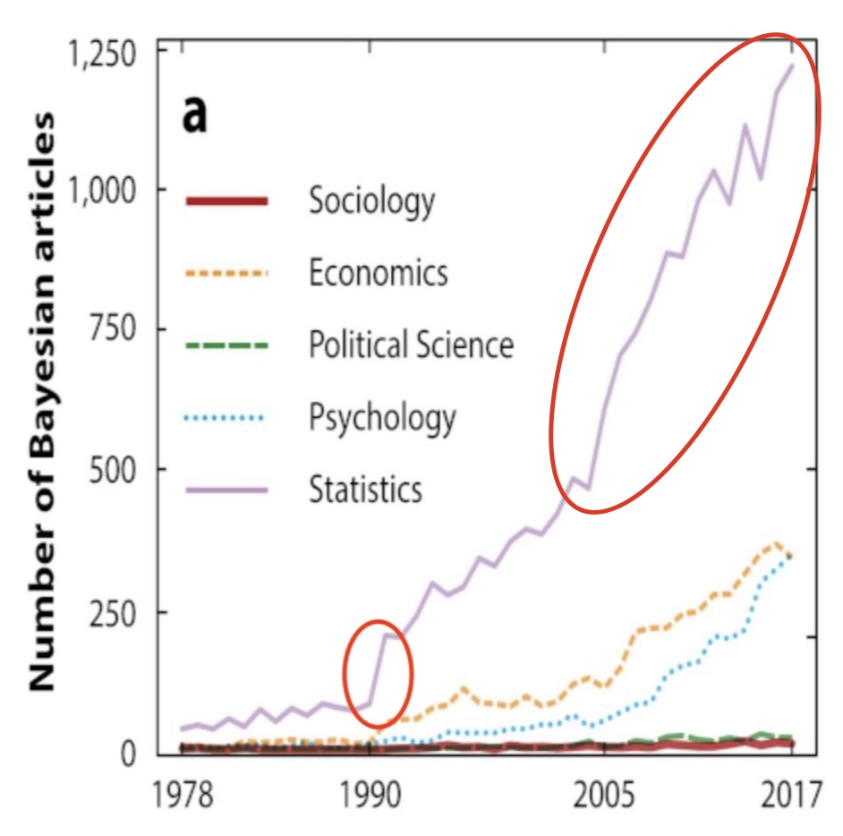
Zooming in
Evolution of probabilistic programming languages: BUGS/JAGS
Bayesian inference Using Gibbs Sampling was one of the first probabilistic programming languages
Flexible syntax allows for definition of (nearly) arbitrary statistical models
Simulation algorithm can sample from (nearly) arbitrary posteriors
Hamstrung by reliance on Gibbs sampling, which doesn’t scale well to high dimensions
Evolution of probabilistic programming languages: Stan
2011: Andrew Gelman’s post-doc Matt Hoffman proposes a modification to an existing MCMC algorithm which allows for sampling from (nearly) arbitrary posteriors
2012: First version of Stan released
Flexible syntax allows for definition of arbitrary statistical models
Scales well to high dimensions due to the “magic” of Hamiltonian Monte Carlo
Stan programs
Bayesian inference and computation
Bayesian inference inextricably linked with computation
Leaps forward in computation allow for more complex models
…which in turn creates more demand for better samplers
Model criticism and comparison
Given that Bayesian inference + modern computation allows for big models, how do we tell if they’re any good?
Posterior predictive checks \[ p(\tilde{y} \mid y) = \int_{\Theta} p(\tilde{y} \mid \theta) p(\theta \mid y) d\theta \]
Leave-one-out cross validation \[ p(\tilde{y}_i \mid y) = \int_{\Theta} p(\tilde{y}_i \mid \theta) p(\theta \mid y_{-i}) d\theta \]
How do we set priors?
Prior predictive checks \[ p(\tilde{y}) = \int_{\Theta} p(\tilde{y} \mid \theta) p(\theta) d\theta \]
To-do for Thursday
Read Chapter 1 in Bayesian Data Analysis
Refresh knowledge of
Probability
PDFs, PMFs, CDFs
Likelihood, Bayes rule