Hierarchical model building

We’ll work through building a hierarchical model for binary data.

First, load the requiste R packages:

library(bayesplot)
library(cmdstanr)
library(posterior)

Now we load the bacteria dataset from the MASS package:

df <- MASS::bacteria 
head(df)

  y ap hilo week  ID     trt
1 y  p   hi    0 X01 placebo
2 y  p   hi    2 X01 placebo
3 y  p   hi    4 X01 placebo
4 y  p   hi   11 X01 placebo
5 y  a   hi    0 X02   drug+
6 y  a   hi    2 X02   drug+

We’ll create a single dataset for the next few exercises in building our Stan models (NB: Stan NOT STAN)

df$idx <- as.integer(df$ID)
df$y <- as.integer(df$y == "y")
des_mat <- model.matrix(~ trt, df)

dat <- 
  list(
    N = nrow(df),
    N_id = length(unique(df$idx)),
    idx = df$idx,
    y = df$y,
    K = ncol(des_mat),
    X = des_mat
  )

First we build a simple Bernoulli model for the data:

data {
  int<lower=0> N;
  array[N] int<lower=0, upper=1> y;

  int<lower=1> N_id;
  array[N] int<lower=1, upper=N_id> idx;
}
parameters {
  real<lower=0, upper=1> theta;
}
model {
  y ~ bernoulli(theta);
}
generated quantities {
  array[N] int y_rep;
  for (n in 1:N)
    y_rep[n] = bernoulli_rng(theta);
}

We then fit this model to our dataset:

fit <- bernoulli$sample(dat)

We’ll look at the posterior predictive check of \(y^{\text{rep}}\) within the patients, defined by the idx column in the data frame.

y_rep <- fit$draws("y_rep", format = "draws_matrix")
bayesplot::ppc_stat_grouped(dat$y, 
                            y_rep,
                            dat$idx,
                            stat = "mean")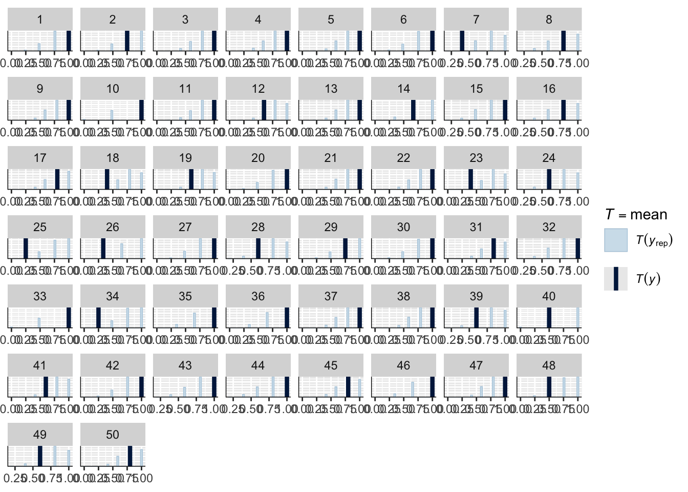

It’s hard to see from this plot, but it looks like there is heterogeneity in the group means that our model isn’t capturing (not surprisingly)

Now let’s add a hierarchy over group-level means to the data. Let \(n_j\) denote the number of observations per patient \(j\) and let \(i\) index the observation within patient.

The model is: \[ \begin{aligned} y_{ij} \mid \theta_j & \sim \text{Bernoulli}(\theta_j)\, \forall i = 1, \dots, n_j \\ \theta_j \mid \alpha, \beta & \sim \text{Beta}(\mu \kappa, (1 - \mu) \kappa) \\ \mu & \sim \text{Unif}(0, 1) \\ 1/\kappa & \sim \text{Cauchy}(0, 1) \end{aligned} \]

data {
  int<lower=0> N;
  array[N] int<lower=0, upper=1> y;

  int<lower=1> N_id;
  array[N] int<lower=1, upper=N_id> idx;
}
parameters {
  vector<lower=0, upper=1>[N_id] theta;
  real<lower=0, upper=1> mu;
  real<lower=0> inv_kappa;
}
transformed parameters {
  // transformation for beta prior
  // (mean, sample size) -> (shape1, shape2)
  real kappa = 1 / inv_kappa;
  real alpha = mu * kappa;
  real beta = (1 - mu) * kappa;
}
model {
  y ~ bernoulli(theta[idx]);
  theta ~ beta(alpha, beta);
  inv_kappa ~ cauchy(0, 1);
}
generated quantities {
  array[N] int y_rep;
  for (n in 1:N)
    y_rep[n] = bernoulli_rng(theta[idx[n]]);
}

We now fit the new model:

fit_hier <- bernoulli_beta_hier$sample(dat, refresh = 2000, seed = 12097807,
                                       iter_sampling = 4000, iter_warmup = 2000)

Running MCMC with 4 sequential chains...

Chain 1 Iteration:    1 / 6000 [  0%]  (Warmup) 
Chain 1 Iteration: 2000 / 6000 [ 33%]  (Warmup) 
Chain 1 Iteration: 2001 / 6000 [ 33%]  (Sampling) 
Chain 1 Iteration: 4000 / 6000 [ 66%]  (Sampling) 
Chain 1 Iteration: 6000 / 6000 [100%]  (Sampling) 
Chain 1 finished in 0.5 seconds.
Chain 2 Iteration:    1 / 6000 [  0%]  (Warmup) 

Chain 2 Informational Message: The current Metropolis proposal is about to be rejected because of the following issue:

Chain 2 Exception: beta_lpdf: Second shape parameter is 0, but must be positive finite! (in '/var/folders/zh/f2m__jwn0g97lbmp2rqv62g00000gn/T/RtmpbHcDEN/model-1565a1a669aab.stan', line 22, column 2 to column 28)

Chain 2 If this warning occurs sporadically, such as for highly constrained variable types like covariance matrices, then the sampler is fine,

Chain 2 but if this warning occurs often then your model may be either severely ill-conditioned or misspecified.

Chain 2 

Chain 2 Informational Message: The current Metropolis proposal is about to be rejected because of the following issue:

Chain 2 Exception: beta_lpdf: Second shape parameter is 0, but must be positive finite! (in '/var/folders/zh/f2m__jwn0g97lbmp2rqv62g00000gn/T/RtmpbHcDEN/model-1565a1a669aab.stan', line 22, column 2 to column 28)

Chain 2 If this warning occurs sporadically, such as for highly constrained variable types like covariance matrices, then the sampler is fine,

Chain 2 but if this warning occurs often then your model may be either severely ill-conditioned or misspecified.

Chain 2 

Chain 2 Informational Message: The current Metropolis proposal is about to be rejected because of the following issue:

Chain 2 Exception: beta_lpdf: Second shape parameter is 0, but must be positive finite! (in '/var/folders/zh/f2m__jwn0g97lbmp2rqv62g00000gn/T/RtmpbHcDEN/model-1565a1a669aab.stan', line 22, column 2 to column 28)

Chain 2 If this warning occurs sporadically, such as for highly constrained variable types like covariance matrices, then the sampler is fine,

Chain 2 but if this warning occurs often then your model may be either severely ill-conditioned or misspecified.

Chain 2 

Chain 2 Iteration: 2000 / 6000 [ 33%]  (Warmup) 
Chain 2 Iteration: 2001 / 6000 [ 33%]  (Sampling) 
Chain 2 Iteration: 4000 / 6000 [ 66%]  (Sampling) 
Chain 2 Iteration: 6000 / 6000 [100%]  (Sampling) 
Chain 2 finished in 0.5 seconds.
Chain 3 Iteration:    1 / 6000 [  0%]  (Warmup) 

Chain 3 Informational Message: The current Metropolis proposal is about to be rejected because of the following issue:

Chain 3 Exception: beta_lpdf: Second shape parameter is 0, but must be positive finite! (in '/var/folders/zh/f2m__jwn0g97lbmp2rqv62g00000gn/T/RtmpbHcDEN/model-1565a1a669aab.stan', line 22, column 2 to column 28)

Chain 3 If this warning occurs sporadically, such as for highly constrained variable types like covariance matrices, then the sampler is fine,

Chain 3 but if this warning occurs often then your model may be either severely ill-conditioned or misspecified.

Chain 3 

Chain 3 Iteration: 2000 / 6000 [ 33%]  (Warmup) 
Chain 3 Iteration: 2001 / 6000 [ 33%]  (Sampling) 
Chain 3 Iteration: 4000 / 6000 [ 66%]  (Sampling) 
Chain 3 Iteration: 6000 / 6000 [100%]  (Sampling) 
Chain 3 finished in 0.5 seconds.
Chain 4 Iteration:    1 / 6000 [  0%]  (Warmup) 
Chain 4 Iteration: 2000 / 6000 [ 33%]  (Warmup) 
Chain 4 Iteration: 2001 / 6000 [ 33%]  (Sampling) 
Chain 4 Iteration: 4000 / 6000 [ 66%]  (Sampling) 
Chain 4 Iteration: 6000 / 6000 [100%]  (Sampling) 
Chain 4 finished in 0.6 seconds.

All 4 chains finished successfully.
Mean chain execution time: 0.5 seconds.
Total execution time: 2.6 seconds.

Warning: 3 of 16000 (0.0%) transitions ended with a divergence.
See https://mc-stan.org/misc/warnings for details.

Warning: 2 of 4 chains had an E-BFMI less than 0.3.
See https://mc-stan.org/misc/warnings for details.

We get this odd error about low-E-BFMI, and some divergences (though depending on your seed you may get more or less than you see above)

We summarize the model:

sum_fit_hier <- fit_hier$summary()
summary(sum_fit_hier$rhat)

   Min. 1st Qu.  Median    Mean 3rd Qu.    Max. 
 0.9998  0.9999  1.0000  1.0001  1.0002  1.0031 

sum_fit_hier[tail(order(sum_fit_hier$rhat)),]

# A tibble: 6 × 10
  variable      mean   median      sd     mad       q5      q95  rhat ess_bulk
  <chr>        <dbl>    <dbl>   <dbl>   <dbl>    <dbl>    <dbl> <dbl>    <dbl>
1 theta[3]     0.911    0.940  0.0919  0.0715    0.721    0.999  1.00    5024.
2 alpha        3.72     3.05   2.62    1.50      1.43     8.04   1.00    1316.
3 inv_kappa    0.285    0.262  0.141   0.128     0.100    0.547  1.00    1241.
4 kappa        4.64     3.82   3.22    1.83      1.83     9.95   1.00    1241.
5 beta         0.921    0.759  0.632   0.357     0.366    1.96   1.00    1123.
6 lp__      -185.    -185.    12.9    12.2    -206.    -164.     1.00     991.
# ℹ 1 more variable: ess_tail <dbl>

Let’s look at some pairs plots to see what’s going on.

We can use bayesplot’s utility functions to pull out the divergent transitions and to plot them along with the pairs plot:

np_pars <- nuts_params(fit_hier)

draws <- fit_hier$draws(format = "draws_array")
bayesplot::mcmc_scatter(draws, pars = c("inv_kappa","theta[21]"), np = np_pars, )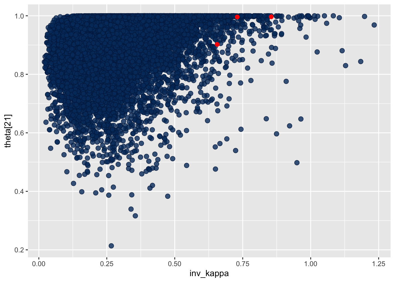

This plot reveals that as inv_kappa grows the posterior gets more concentrated around \(1\) for \(\theta_{21}\), which can lead to numerical instability (remember about how numbers near 1 are less precise in floating point compared to numbers near \(0\)?).

Let’s look at the logit of \(\theta_{21}\)

bayesplot::mcmc_scatter(draws, pars = c("inv_kappa","theta[21]"), np = np_pars, transformations = list("theta[21]"=qlogis))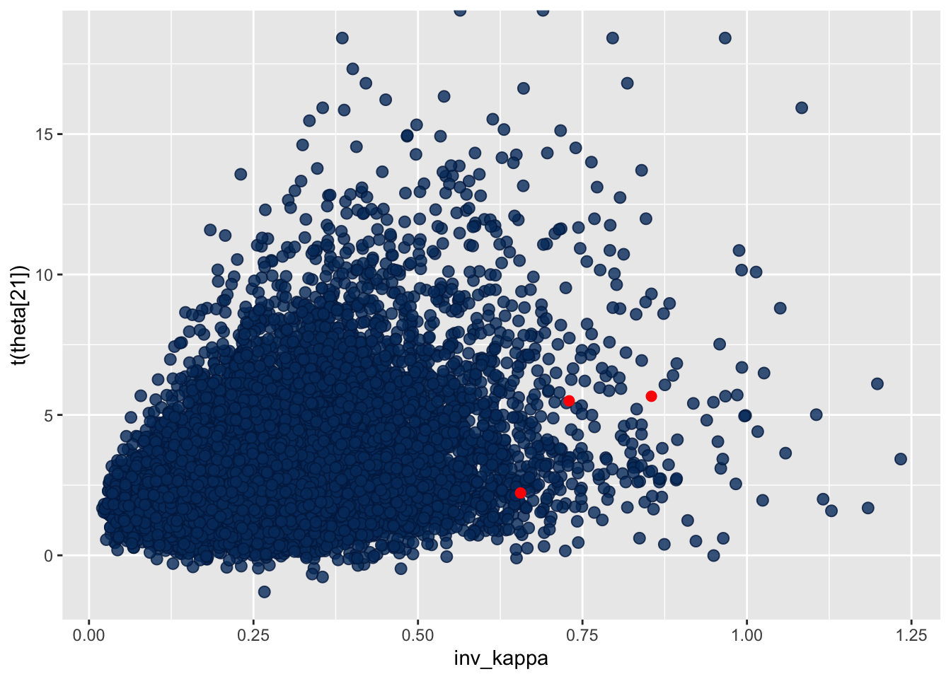

Let’s try to reparameterize to see if we can address the problem. This will be a class exercise.

Using the hierarchical model you’ve built above, write the following model

\[ \begin{aligned} y_{ij} \mid \theta_j & \sim \text{Bernoulli}(\theta_j)\, \forall i = 1, \dots, n_j \\ \eta_j \mid \mu_\eta, \tau & \sim \text{Normal}(\mu_\eta, \tau^2) \\ \theta_j & = \text{inv\_logit}(\eta_j) \\ \mu & \sim \text{Unif}(0,1) \\ \mu_\eta & = \text{logit}(\mu) \\ \tau & \sim \text{Normal}(0, 5) \end{aligned} \] Depending on how you parameterize the hierarchy over \(\eta_j\), you may get divergences. If so, use the same strategy as above to plot a specific \(\eta\) parameter vs. \(\tau\). For visualization purposes it can be helpful to plot \(\log \tau\) instead of \(\tau\).

data {
  int<lower=0> N;
  array[N] int<lower=0, upper=1> y;

  int<lower=1> N_id;
  array[N] int<lower=1, upper=N_id> idx;
}
parameters {
  vector[N_id] eta;
  real<lower=0, upper=1> mu;
  real<lower=0> tau;
}
transformed parameters {
  // transformation for beta prior
  // (mean, sample size) -> (shape1, shape2)
  vector[N_id] theta = inv_logit(eta);
}
model {
  y ~ bernoulli(theta[idx]);
  eta ~ normal(logit(mu), tau);
  tau ~ normal(0, 5);
}
generated quantities {
  array[N] int y_rep;
  for (n in 1:N)
    y_rep[n] = bernoulli_rng(theta[idx[n]]);
}

fit_norm <- bernoulli_norm_hier$sample(dat, refresh = 2000, seed = 12097807,
                                       iter_sampling = 4000, iter_warmup = 2000)

Running MCMC with 4 sequential chains...

Chain 1 Iteration:    1 / 6000 [  0%]  (Warmup) 
Chain 1 Iteration: 2000 / 6000 [ 33%]  (Warmup) 
Chain 1 Iteration: 2001 / 6000 [ 33%]  (Sampling) 
Chain 1 Iteration: 4000 / 6000 [ 66%]  (Sampling) 
Chain 1 Iteration: 6000 / 6000 [100%]  (Sampling) 
Chain 1 finished in 0.4 seconds.
Chain 2 Iteration:    1 / 6000 [  0%]  (Warmup) 

Chain 2 Informational Message: The current Metropolis proposal is about to be rejected because of the following issue:

Chain 2 Exception: normal_lpdf: Location parameter is inf, but must be finite! (in '/var/folders/zh/f2m__jwn0g97lbmp2rqv62g00000gn/T/RtmpOmeQ3R/model-173bd61668f51.stan', line 20, column 2 to column 31)

Chain 2 If this warning occurs sporadically, such as for highly constrained variable types like covariance matrices, then the sampler is fine,

Chain 2 but if this warning occurs often then your model may be either severely ill-conditioned or misspecified.

Chain 2 

Chain 2 Informational Message: The current Metropolis proposal is about to be rejected because of the following issue:

Chain 2 Exception: normal_lpdf: Location parameter is inf, but must be finite! (in '/var/folders/zh/f2m__jwn0g97lbmp2rqv62g00000gn/T/RtmpOmeQ3R/model-173bd61668f51.stan', line 20, column 2 to column 31)

Chain 2 If this warning occurs sporadically, such as for highly constrained variable types like covariance matrices, then the sampler is fine,

Chain 2 but if this warning occurs often then your model may be either severely ill-conditioned or misspecified.

Chain 2 

Chain 2 Informational Message: The current Metropolis proposal is about to be rejected because of the following issue:

Chain 2 Exception: normal_lpdf: Location parameter is inf, but must be finite! (in '/var/folders/zh/f2m__jwn0g97lbmp2rqv62g00000gn/T/RtmpOmeQ3R/model-173bd61668f51.stan', line 20, column 2 to column 31)

Chain 2 If this warning occurs sporadically, such as for highly constrained variable types like covariance matrices, then the sampler is fine,

Chain 2 but if this warning occurs often then your model may be either severely ill-conditioned or misspecified.

Chain 2 

Chain 2 Informational Message: The current Metropolis proposal is about to be rejected because of the following issue:

Chain 2 Exception: normal_lpdf: Location parameter is inf, but must be finite! (in '/var/folders/zh/f2m__jwn0g97lbmp2rqv62g00000gn/T/RtmpOmeQ3R/model-173bd61668f51.stan', line 20, column 2 to column 31)

Chain 2 If this warning occurs sporadically, such as for highly constrained variable types like covariance matrices, then the sampler is fine,

Chain 2 but if this warning occurs often then your model may be either severely ill-conditioned or misspecified.

Chain 2 

Chain 2 Informational Message: The current Metropolis proposal is about to be rejected because of the following issue:

Chain 2 Exception: normal_lpdf: Location parameter is inf, but must be finite! (in '/var/folders/zh/f2m__jwn0g97lbmp2rqv62g00000gn/T/RtmpOmeQ3R/model-173bd61668f51.stan', line 20, column 2 to column 31)

Chain 2 If this warning occurs sporadically, such as for highly constrained variable types like covariance matrices, then the sampler is fine,

Chain 2 but if this warning occurs often then your model may be either severely ill-conditioned or misspecified.

Chain 2 

Chain 2 Informational Message: The current Metropolis proposal is about to be rejected because of the following issue:

Chain 2 Exception: normal_lpdf: Location parameter is inf, but must be finite! (in '/var/folders/zh/f2m__jwn0g97lbmp2rqv62g00000gn/T/RtmpOmeQ3R/model-173bd61668f51.stan', line 20, column 2 to column 31)

Chain 2 If this warning occurs sporadically, such as for highly constrained variable types like covariance matrices, then the sampler is fine,

Chain 2 but if this warning occurs often then your model may be either severely ill-conditioned or misspecified.

Chain 2 

Chain 2 Iteration: 2000 / 6000 [ 33%]  (Warmup) 
Chain 2 Iteration: 2001 / 6000 [ 33%]  (Sampling) 
Chain 2 Iteration: 4000 / 6000 [ 66%]  (Sampling) 
Chain 2 Iteration: 6000 / 6000 [100%]  (Sampling) 
Chain 2 finished in 0.5 seconds.
Chain 3 Iteration:    1 / 6000 [  0%]  (Warmup) 
Chain 3 Iteration: 2000 / 6000 [ 33%]  (Warmup) 
Chain 3 Iteration: 2001 / 6000 [ 33%]  (Sampling) 

Chain 3 Informational Message: The current Metropolis proposal is about to be rejected because of the following issue:

Chain 3 Exception: normal_lpdf: Location parameter is -inf, but must be finite! (in '/var/folders/zh/f2m__jwn0g97lbmp2rqv62g00000gn/T/RtmpOmeQ3R/model-173bd61668f51.stan', line 20, column 2 to column 31)

Chain 3 If this warning occurs sporadically, such as for highly constrained variable types like covariance matrices, then the sampler is fine,

Chain 3 but if this warning occurs often then your model may be either severely ill-conditioned or misspecified.

Chain 3 

Chain 3 Iteration: 4000 / 6000 [ 66%]  (Sampling) 
Chain 3 Iteration: 6000 / 6000 [100%]  (Sampling) 
Chain 3 finished in 0.6 seconds.
Chain 4 Iteration:    1 / 6000 [  0%]  (Warmup) 

Chain 4 Informational Message: The current Metropolis proposal is about to be rejected because of the following issue:

Chain 4 Exception: normal_lpdf: Location parameter is -inf, but must be finite! (in '/var/folders/zh/f2m__jwn0g97lbmp2rqv62g00000gn/T/RtmpOmeQ3R/model-173bd61668f51.stan', line 20, column 2 to column 31)

Chain 4 If this warning occurs sporadically, such as for highly constrained variable types like covariance matrices, then the sampler is fine,

Chain 4 but if this warning occurs often then your model may be either severely ill-conditioned or misspecified.

Chain 4 

Chain 4 Iteration: 2000 / 6000 [ 33%]  (Warmup) 
Chain 4 Iteration: 2001 / 6000 [ 33%]  (Sampling) 
Chain 4 Iteration: 4000 / 6000 [ 66%]  (Sampling) 
Chain 4 Iteration: 6000 / 6000 [100%]  (Sampling) 
Chain 4 finished in 0.5 seconds.

All 4 chains finished successfully.
Mean chain execution time: 0.5 seconds.
Total execution time: 2.3 seconds.

Warning: 2 of 16000 (0.0%) transitions ended with a divergence.
See https://mc-stan.org/misc/warnings for details.

Warning: 4 of 4 chains had an E-BFMI less than 0.3.
See https://mc-stan.org/misc/warnings for details.

np_pars <- nuts_params(fit_norm)

draws <- fit_norm$draws(format = "draws_array")
bayesplot::mcmc_scatter(draws, pars = c("eta[21]","tau"), np = np_pars, transformations = list("tau" = log))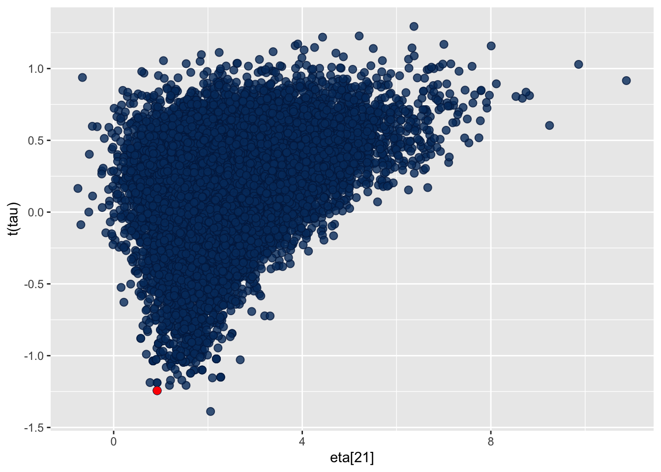

Reparameterization

\[ \begin{aligned} y_{ij} \mid \theta_j & \sim \text{Bernoulli}(\theta_j)\, \forall i = 1, \dots, n_j \\ \eta_j & \sim \text{Normal}(0, 1) \\ \theta_j & = \text{inv\_logit}(\mu_\eta + \tau \eta_j) \\ \mu & \sim \text{Unif}(0,1) \\ \mu_\eta & = \text{logit}(\mu) \\ \tau & \sim \text{Normal}(0, 5) \end{aligned} \]

data {
  int<lower=0> N;
  array[N] int<lower=0, upper=1> y;

  int<lower=1> N_id;
  array[N] int<lower=1, upper=N_id> idx;
}
parameters {
  vector[N_id] eta;
  real<lower=0, upper=1> mu;
  real<lower=0> tau;
}
transformed parameters {
  // transformation for beta prior
  // (mean, sample size) -> (shape1, shape2)
  vector[N_id] theta = inv_logit(logit(mu) + tau * eta);
}
model {
  y ~ bernoulli(theta[idx]);
  eta ~ std_normal();
  tau ~ normal(0, 5);
}
generated quantities {
  array[N] int y_rep;
  for (n in 1:N)
    y_rep[n] = bernoulli_rng(theta[idx[n]]);
}

fit_ncp <- bernoulli_norm_hier_ncp$sample(dat, refresh = 2000, seed = 12097807,
                                       iter_sampling = 4000, iter_warmup = 2000)

Running MCMC with 4 sequential chains...

Chain 1 Iteration:    1 / 6000 [  0%]  (Warmup) 
Chain 1 Iteration: 2000 / 6000 [ 33%]  (Warmup) 
Chain 1 Iteration: 2001 / 6000 [ 33%]  (Sampling) 
Chain 1 Iteration: 4000 / 6000 [ 66%]  (Sampling) 
Chain 1 Iteration: 6000 / 6000 [100%]  (Sampling) 
Chain 1 finished in 0.5 seconds.
Chain 2 Iteration:    1 / 6000 [  0%]  (Warmup) 
Chain 2 Iteration: 2000 / 6000 [ 33%]  (Warmup) 
Chain 2 Iteration: 2001 / 6000 [ 33%]  (Sampling) 
Chain 2 Iteration: 4000 / 6000 [ 66%]  (Sampling) 
Chain 2 Iteration: 6000 / 6000 [100%]  (Sampling) 
Chain 2 finished in 0.5 seconds.
Chain 3 Iteration:    1 / 6000 [  0%]  (Warmup) 
Chain 3 Iteration: 2000 / 6000 [ 33%]  (Warmup) 
Chain 3 Iteration: 2001 / 6000 [ 33%]  (Sampling) 
Chain 3 Iteration: 4000 / 6000 [ 66%]  (Sampling) 
Chain 3 Iteration: 6000 / 6000 [100%]  (Sampling) 
Chain 3 finished in 0.5 seconds.
Chain 4 Iteration:    1 / 6000 [  0%]  (Warmup) 
Chain 4 Iteration: 2000 / 6000 [ 33%]  (Warmup) 
Chain 4 Iteration: 2001 / 6000 [ 33%]  (Sampling) 
Chain 4 Iteration: 4000 / 6000 [ 66%]  (Sampling) 
Chain 4 Iteration: 6000 / 6000 [100%]  (Sampling) 
Chain 4 finished in 0.5 seconds.

All 4 chains finished successfully.
Mean chain execution time: 0.5 seconds.
Total execution time: 2.2 seconds.

np_pars <- nuts_params(fit_ncp)

draws <- fit_ncp$draws(format = "draws_array")
bayesplot::mcmc_scatter(draws, pars = c("eta[21]","tau"), np = np_pars, transformations = list("tau" = log))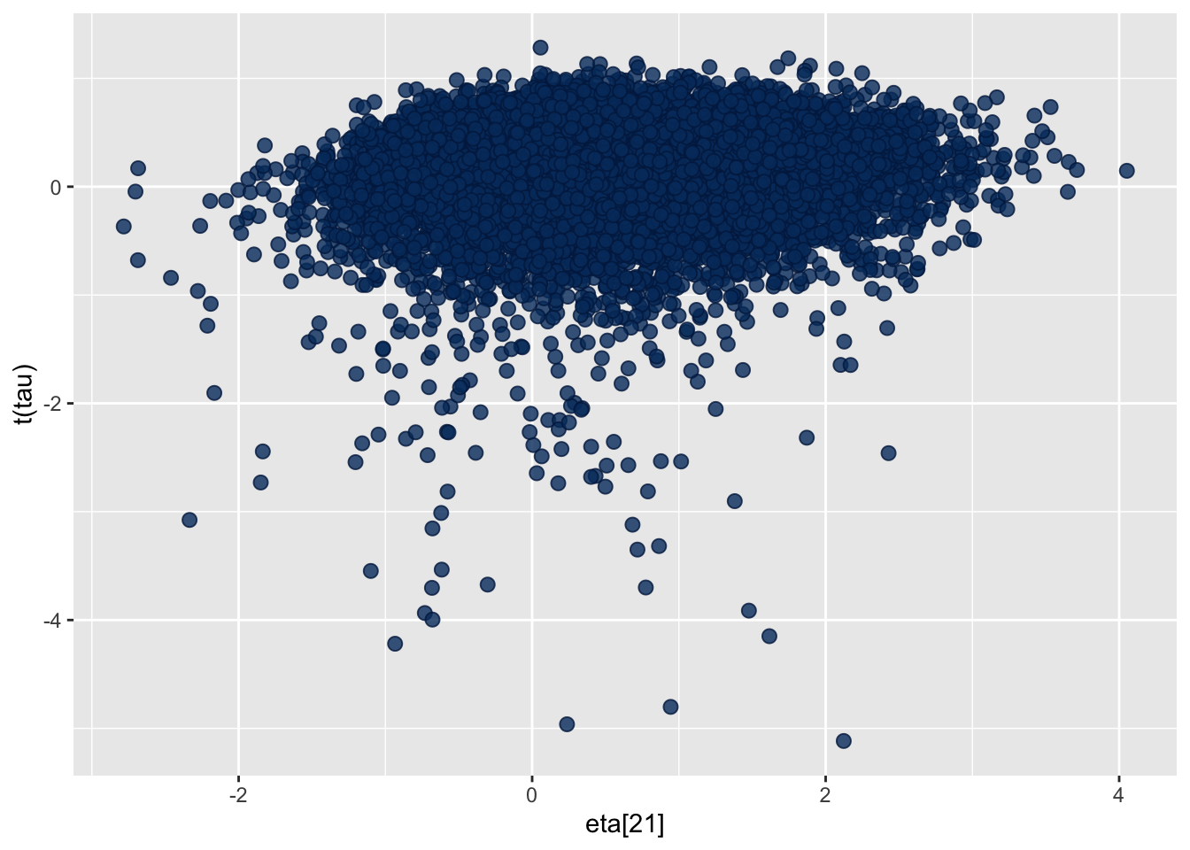

\[ \begin{aligned} y_{ij} \mid \theta_j & \sim \text{Bernoulli}(\theta_{ij})\, \forall i = 1, \dots, n_j \\ \eta_j & \sim \text{Normal}(0, 1) \\ \theta_{ij} & = \text{inv\_logit}(X_{ij}^T \beta + \tau \eta_j) \\ \beta & = \text{Normal}(0, 5) \\ \tau & \sim \text{Normal}(0, 5) \end{aligned} \]

data {
  int<lower=0> N;
  array[N] int<lower=0, upper=1> y;

  int<lower=1> N_id;
  array[N] int<lower=1, upper=N_id> idx;
  
  int<lower=1> K;
  matrix[N, K] X;
}
parameters {
  vector[N_id] eta;
  vector[K] beta;
  real<lower=0> tau;
}
transformed parameters {
  // transformation for beta prior
  // (mean, sample size) -> (shape1, shape2)
  vector[N_id] eta_scale = tau * eta;
}
model {
  vector[N] lin_pred = X * beta;
  y ~ bernoulli_logit(lin_pred + eta_scale[idx]);
  eta ~ std_normal();
  tau ~ normal(0, 5);
  beta ~ normal(0, 5);
}
generated quantities {
  array[N] int y_rep;
  {
  vector[N] theta = inv_logit(X * beta + eta_scale[idx]);
  for (n in 1:N)
    y_rep[n] = bernoulli_rng(theta[n]);
  }
}

fit_ncp_reg <- bernoulli_norm_hier_ncp_reg$sample(dat, refresh = 2000, seed = 12097807,
                                       iter_sampling = 4000, iter_warmup = 2000)

Running MCMC with 4 sequential chains...

Chain 1 Iteration:    1 / 6000 [  0%]  (Warmup) 
Chain 1 Iteration: 2000 / 6000 [ 33%]  (Warmup) 
Chain 1 Iteration: 2001 / 6000 [ 33%]  (Sampling) 
Chain 1 Iteration: 4000 / 6000 [ 66%]  (Sampling) 
Chain 1 Iteration: 6000 / 6000 [100%]  (Sampling) 
Chain 1 finished in 0.8 seconds.
Chain 2 Iteration:    1 / 6000 [  0%]  (Warmup) 
Chain 2 Iteration: 2000 / 6000 [ 33%]  (Warmup) 
Chain 2 Iteration: 2001 / 6000 [ 33%]  (Sampling) 
Chain 2 Iteration: 4000 / 6000 [ 66%]  (Sampling) 
Chain 2 Iteration: 6000 / 6000 [100%]  (Sampling) 
Chain 2 finished in 0.8 seconds.
Chain 3 Iteration:    1 / 6000 [  0%]  (Warmup) 
Chain 3 Iteration: 2000 / 6000 [ 33%]  (Warmup) 
Chain 3 Iteration: 2001 / 6000 [ 33%]  (Sampling) 
Chain 3 Iteration: 4000 / 6000 [ 66%]  (Sampling) 
Chain 3 Iteration: 6000 / 6000 [100%]  (Sampling) 
Chain 3 finished in 0.8 seconds.
Chain 4 Iteration:    1 / 6000 [  0%]  (Warmup) 
Chain 4 Iteration: 2000 / 6000 [ 33%]  (Warmup) 
Chain 4 Iteration: 2001 / 6000 [ 33%]  (Sampling) 
Chain 4 Iteration: 4000 / 6000 [ 66%]  (Sampling) 
Chain 4 Iteration: 6000 / 6000 [100%]  (Sampling) 
Chain 4 finished in 1.0 seconds.

All 4 chains finished successfully.
Mean chain execution time: 0.8 seconds.
Total execution time: 3.6 seconds.

sum_fit <- fit_ncp_reg$summary()
sum_fit[tail(order(sum_fit$rhat)),]

# A tibble: 6 × 10
  variable          mean   median    sd   mad       q5      q95  rhat ess_bulk
  <chr>            <dbl>    <dbl> <dbl> <dbl>    <dbl>    <dbl> <dbl>    <dbl>
1 eta[18]         -0.799   -0.799 0.664 0.634   -1.87     0.277  1.00   17739.
2 eta_scale[43]    0.581    0.466 1.16  1.04    -1.12     2.65   1.00   20652.
3 eta_scale[36]    0.795    0.680 1.13  1.03    -0.851    2.79   1.00   16355.
4 eta_scale[44]    1.04     0.904 1.13  1.01    -0.531    3.07   1.00   12447.
5 lp__          -115.    -115.    7.87  7.79  -129.    -103.     1.00    2872.
6 tau              1.30     1.27  0.457 0.435    0.605    2.09   1.00    3269.
# ℹ 1 more variable: ess_tail <dbl>

time <- fit_ncp_reg$time()$total
ess_p_sec <- summary(sum_fit$ess_bulk / time)

hist(fit_ncp_reg$draws("beta[2]",format = "draws_matrix"),
     main = "Posterior effect of treatment 1",
     xlab = bquote(beta[2]))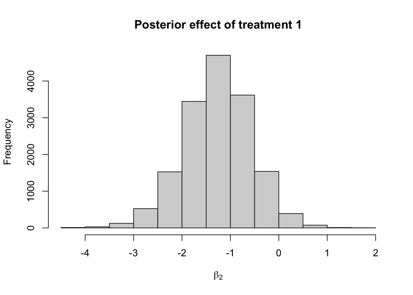

hist(fit_ncp_reg$draws("beta[3]",format = "draws_matrix"),
     main = "Posterior effect of treatment 2",
      xlab = bquote(beta[3]))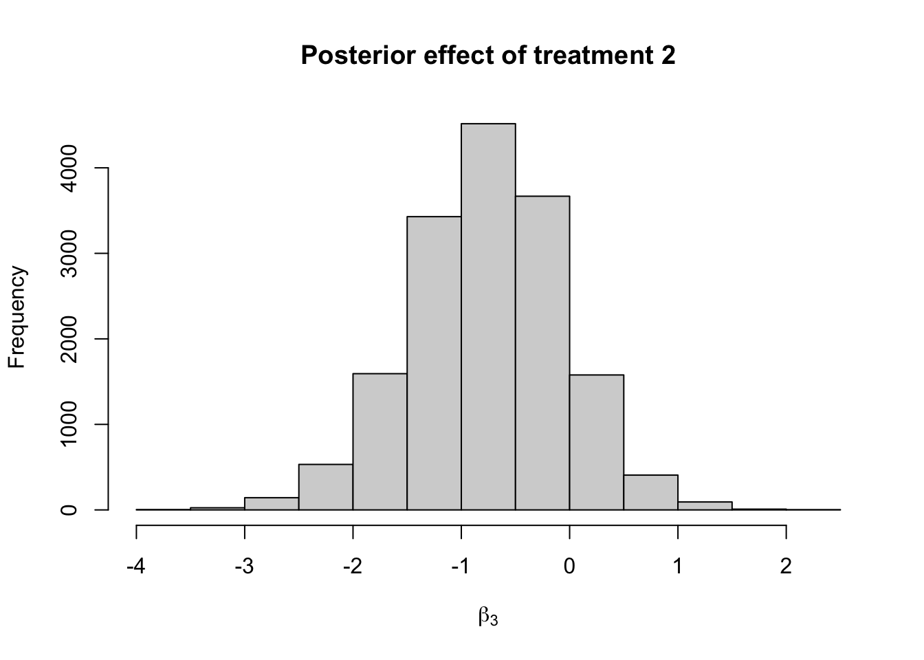

hist(fit_ncp_reg$draws("beta[2]",format = "draws_matrix") - fit_ncp_reg$draws("beta[3]",format = "draws_matrix"),
     main = "Difference between treatments",
     xlab = bquote(beta[2]-beta[3]))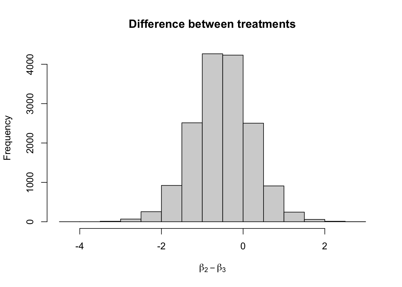

One final iteration of our model uses the bernoulli_logit_glm function, which takes a matrix of covariates, a vector of means on the logit scale of length equal to the number of rows in the matrix of covariates, and a vector of covariates.

data {
  int<lower=0> N;
  array[N] int<lower=0, upper=1> y;

  int<lower=1> N_id;
  array[N] int<lower=1, upper=N_id> idx;
  
  int<lower=1> K;
  matrix[N, K] X;
}
parameters {
  vector[N_id] eta;
  vector[K] beta;
  real<lower=0> tau;
}
transformed parameters {
  // transformation for beta prior
  // (mean, sample size) -> (shape1, shape2)
  vector[N_id] eta_scale = tau * eta;
}
model {
  y ~ bernoulli_logit_glm(X, eta_scale[idx], beta);
  eta ~ std_normal();
  tau ~ normal(0, 5);
  beta ~ normal(0, 5);
}
generated quantities {
  array[N] int y_rep;
  {
  vector[N] theta = inv_logit(X * beta + eta_scale[idx]);
  for (n in 1:N)
    y_rep[n] = bernoulli_rng(theta[n]);
  }
}

fit_ncp_glm <- bernoulli_logit_glm_norm_hier_ncp$sample(dat, refresh = 2000, seed = 12097807,
                                       iter_sampling = 4000, iter_warmup = 2000)

Running MCMC with 4 sequential chains...

Chain 1 Iteration:    1 / 6000 [  0%]  (Warmup) 
Chain 1 Iteration: 2000 / 6000 [ 33%]  (Warmup) 
Chain 1 Iteration: 2001 / 6000 [ 33%]  (Sampling) 
Chain 1 Iteration: 4000 / 6000 [ 66%]  (Sampling) 
Chain 1 Iteration: 6000 / 6000 [100%]  (Sampling) 
Chain 1 finished in 0.6 seconds.
Chain 2 Iteration:    1 / 6000 [  0%]  (Warmup) 
Chain 2 Iteration: 2000 / 6000 [ 33%]  (Warmup) 
Chain 2 Iteration: 2001 / 6000 [ 33%]  (Sampling) 
Chain 2 Iteration: 4000 / 6000 [ 66%]  (Sampling) 
Chain 2 Iteration: 6000 / 6000 [100%]  (Sampling) 
Chain 2 finished in 0.6 seconds.
Chain 3 Iteration:    1 / 6000 [  0%]  (Warmup) 
Chain 3 Iteration: 2000 / 6000 [ 33%]  (Warmup) 
Chain 3 Iteration: 2001 / 6000 [ 33%]  (Sampling) 
Chain 3 Iteration: 4000 / 6000 [ 66%]  (Sampling) 
Chain 3 Iteration: 6000 / 6000 [100%]  (Sampling) 
Chain 3 finished in 0.6 seconds.
Chain 4 Iteration:    1 / 6000 [  0%]  (Warmup) 
Chain 4 Iteration: 2000 / 6000 [ 33%]  (Warmup) 
Chain 4 Iteration: 2001 / 6000 [ 33%]  (Sampling) 
Chain 4 Iteration: 4000 / 6000 [ 66%]  (Sampling) 
Chain 4 Iteration: 6000 / 6000 [100%]  (Sampling) 
Chain 4 finished in 0.6 seconds.

All 4 chains finished successfully.
Mean chain execution time: 0.6 seconds.
Total execution time: 2.7 seconds.

sum_fit <- fit_ncp_glm$summary()
sum_fit[tail(order(sum_fit$rhat)),]

# A tibble: 6 × 10
  variable          mean   median    sd   mad       q5      q95  rhat ess_bulk
  <chr>            <dbl>    <dbl> <dbl> <dbl>    <dbl>    <dbl> <dbl>    <dbl>
1 eta[18]         -0.799   -0.799 0.664 0.634   -1.87     0.277  1.00   17739.
2 eta_scale[43]    0.581    0.466 1.16  1.04    -1.12     2.65   1.00   20652.
3 eta_scale[36]    0.795    0.680 1.13  1.03    -0.851    2.79   1.00   16355.
4 eta_scale[44]    1.04     0.904 1.13  1.01    -0.531    3.07   1.00   12447.
5 lp__          -115.    -115.    7.87  7.79  -129.    -103.     1.00    2872.
6 tau              1.30     1.27  0.457 0.435    0.605    2.09   1.00    3269.
# ℹ 1 more variable: ess_tail <dbl>

time <- fit_ncp_glm$time()$total
ess_p_sec_glm <- summary(sum_fit$ess_bulk / time)

Using the bernoulli_logit_glm results in higher effective sample size per second:

round(cbind(ess_p_sec_glm, ess_p_sec))

        ess_p_sec_glm ess_p_sec
Min.             1062       801
1st Qu.          5769      4354
Median           5981      4514
Mean             6158      4647
3rd Qu.          6275      4736
Max.             9462      7141