---
title: "Lab 3"
format:
html:
html-math-method:
method: mathjax
url: "https://cdn.jsdelivr.net/npm/mathjax@4.1/tex-mml-chtml.js"
include-in-header:
text: |
<script>
window.MathJax = {
startup: {
ready() {
MathJax.startup.defaultReady();
const {STATE} = MathJax._.core.MathItem;
MathJax.tex2mml(String.raw`
\newcommand{\lp}{\left(}
\newcommand{\rp}{\right)}
\newcommand{\R}{\mathbb{R}}
\newcommand{\Z}{\mathbb{Z}}
\newcommand{\lb}{\left[}
\newcommand{\rb}{\right]}
\newcommand{\ind}[1]{\mathbbm{1}\lp#1\rp}
\newcommand{\Exp}[1]{\mathbb{E} \lb #1 \rb}
\newcommand{\ExpA}[2]{\mathbb{E}_{#2} \lb #1 \rb}
\newcommand{\Prob}[2]{\mathbb{P}_{#2} \lp #1 \rp}
\newcommand{\indy}{\mathrel{\unicode{x2AEB}}}
\newcommand{\comp}{^\mathsf{c}}
\newcommand{\widebar}[1]{\overline{\! #1}}
\newcommand{\Var}[1]{\mathrm{Var}\lp #1 \rp}
\newcommand{\Cov}[2]{\mathrm{Cov}\lp #1,#2 \rp}
\newcommand{\VarA}[2]{\mathrm{Var}_{#2}\lp #1 \rp}
\newcommand{\norm}[1]{\left\lVert #1 \right\rVert}
\newcommand{\ddtA}[1]{\frac{\partial^2}{\partial #1^2}}
\newcommand{\ddtB}[2]{\frac{\partial^2}{\partial #1 \partial #2}}
\newcommand{\diff}[1]{{\mathrm{d}}\!\lp #1 \rp}
\newcommand{\veco}[1]{{\mathrm{vec}}\lp #1 \rp}
\newcommand{\tr}[1]{{\mathrm{tr}}\lp #1 \rp}
`);
}
},
loader: {load: ['[tex]/bbm','[tex]/upgreek']},
tex: {packages: {'[+]': ['bbm','upgreek']}}
};
</script>
code-tools:
source: true
toggle: false
caption: "Download Source"
---
# Summary
This lab will explore mixture importance sampling.
## Importance sampling
Let's say we have an observation, $x_1$, from the following Bayesian model: $$
\begin{aligned}
X_1 \mid \theta & \sim t_{4}(\theta, 1) \\
\theta & \sim t_{2}(0, 1)
\end{aligned}
$$ and we wish to estimate the posterior mean:
$$
\Exp{\theta \mid X_1 = x_1}
$$
We know from class that the posterior distribution, which we'll denote as $\pi(\theta \mid x_1)$ is proportional to the likelihood, denoted $L(\theta \mid x_1)$ times the prior, $\pi(\theta)$.
In this case: $$
\begin{aligned}
L(\theta \mid x_1) & \propto \left(1 + \frac{1}{4}(x_1 - \theta)^2\right)^{-5/2} \\
\pi(\theta) & \propto \left(1 + \frac{\theta^2}{2}\right)^{-3/2} \\
\end{aligned}
$$ Then the posterior is
$$
\begin{aligned}
\pi(\theta \mid x_1) \propto \left(1 + \frac{1}{4}(x_1 - \theta)^2\right)^{-5/2}\left(1 + \frac{\theta^2}{2}\right)^{-3/2}
\end{aligned}
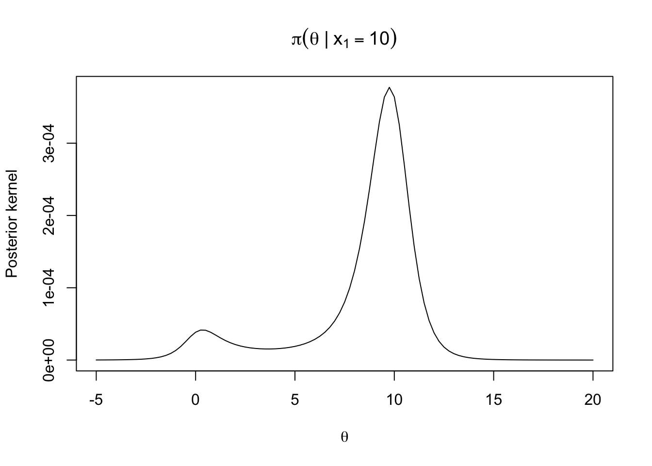
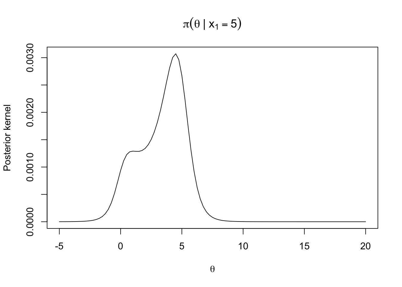
$$ Let's plot this below for $x_1 = 10$ and for $x_1 = 5$
```{r}
x_1 <- 10
log_post_prop <- function(theta, x_1) {
  dt(x_1 - theta, df = 4, log = TRUE) + dt(theta, df = 2, log = TRUE)
}

post_prop <- function(theta, x_1){exp(log_post_prop(theta, x_1))}

curve(post_prop(x, x_1), from = -5, to = 20, main = bquote(pi(theta~"|"~x[1]==10)),
      xlab = bquote(theta), ylab = "Posterior kernel")
```
```{r}
curve(post_prop(x, 5), from = -5, to = 20, main = bquote(pi(theta~"|"~x[1]==5)),
      xlab = bquote(theta), ylab = "Posterior kernel")
```
Let's use mixture self-normalized importance sampling to estimate the posterior mean with $f_u(\theta) = \pi(\theta \mid x_1)$ up to a constant of proportionality.
$$
\tilde{\mu}_{\text{IS}} = \sum_{i=1}^Sw(\theta_i) h(\theta_i)
$$ where $$
w(\theta_i) = \frac{f_u(\theta_i)/g(\theta_i)}{\sum_{j=1}^S f_u(\theta_j)/g(\theta_j)}
$$ and $h(\theta_i) = \theta_i$.
We'll pull forward the `log_sum_exp` function we defined in [Lab 2](Lab-2.qmd):
```{r}
log_sum_exp <- function(x) {
  max_x <- max(x)
  return(max_x + log(sum(exp(x - max_x))))
}
```
and we'll use $$
g(\theta) = 0.3 \left(1 + \frac{\theta^2}{2}\right)^{-3/2} + 0.7 \left(1 + \frac{1}{4}(\theta - x_1)^2\right)^{-5/2}
$$
as our proposal density.
We can generate samples from this using the following procedure: $$
\begin{aligned}
& \text{For } i = 1, \dots, S \\
W_i & \sim \text{Bernoulli}(0.3) \\
\theta_i & \sim
\begin{cases}
t_2(0,1) & W_i = 1 \\
t_4(x_1,1) & W_i = 0
\end{cases}
\end{aligned}
$$
## Your turn
Write an R function, `importance_samples`, that takes the arguments, `S` and `x`, and returns a vector of draws `theta` according to the model above. It will help to remember that the $t$ distribution is a location family, so $\theta \sim t_{\text{df}}(\mu,1)$ is equal in distribution to $$
Z \sim t_\text{df}(0,1), \, \theta = \mu + Z
$$
```{r}
#| eval: false
importance_samples <- function(S, x) {
  theta <-
  return(theta)
}
```
## Defining a function to evaluate $g(\theta)$
Now we need to evaluate the importance weights. We already have a function that defines the log of the kernel of the posterior, called `log_post_prop`.
## Your turn
Write a function that defines the log of the importance density as defined above. You'll need to use `dt` as it is used above and include the appropriate weights.
The function is called `log_g` and it will take a vector `theta` and a scalar `x` and return a vector of the log of the importance density evaluated at `theta`
```{r}
log_g <- function(theta, x) {
  ###
  return(log_g_eval)
}
```
### Challenge
How can you use the function `log_sum_exp` to generate the log of the importance density?
## Log importance weights
Now that you have functions that can generate importance samples and evaluate the importance density at those draws, we can evaluate the log-importance weights.
## Your turn
1. For the $x_1 = 10$ scenario, generate $1{,}000$ draws of $\theta$ from $g$, and assign to `theta_draws`
2. Evaluate the kernel of the log-posterior at your draws for $\theta$ using `log_post_prop`, and assign to `log_post_draws`
3. Evaluate the log of importance density at your draws for $\theta$, and assign to `log_g_draws`
4. Calculate the `log_weights` as indicated below
Fill in the following code:
```{r}
#| eval: false
theta_draws <-
log_post_draws <-
log_g_draws <-
num <- log_post_draws - log_g_draws
log_weights <- num - log_sum_exp(num)
```
Now we can **finally** estimate the posterior mean.:
$$
\hat{\Exp{\theta \mid X_1 = x_1}} \approx \tilde{\mu}_\text{IS}
$$ where
$$
\tilde{\mu}_\text{IS} = \sum_{i=1}^S \exp(\log w(\theta_i)) \theta_i
$$
```{r}
#| eval: false
approx_post_mean <-
```
## Evaluating the variance of our estimate
Using the [formula](../lectures/Lecture-4-Importance-Sampling.qmd#eq-var-snis) for the variance of self-normalized importance sampling example we can estimate how precise our estimate of the mean is.
This is
```{r}
#| eval: false
sq_weights <- exp(2 * log_weights)
var_est <- sum(sq_weights * (theta_draws - approx_post_mean)^2)
```