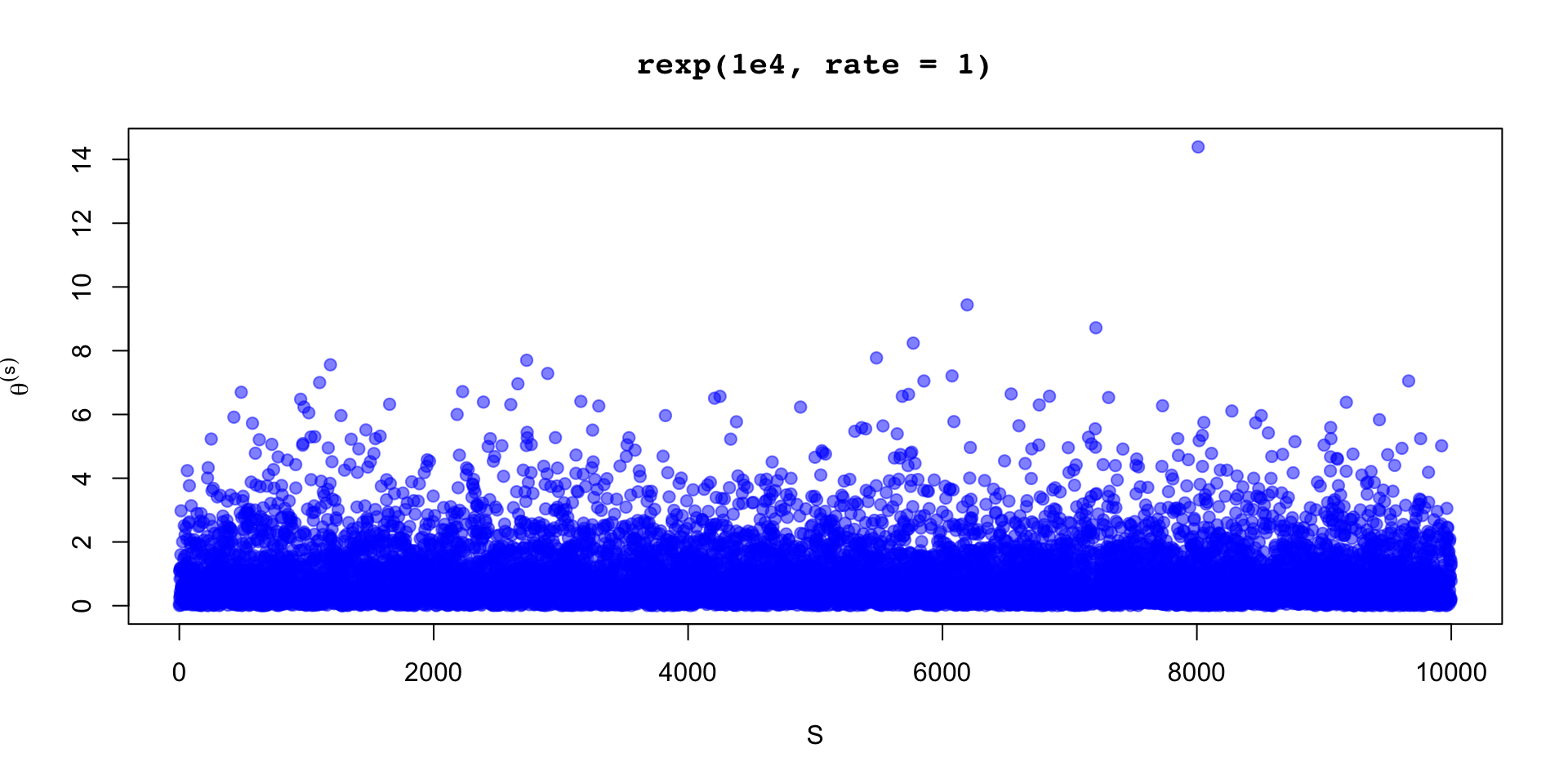
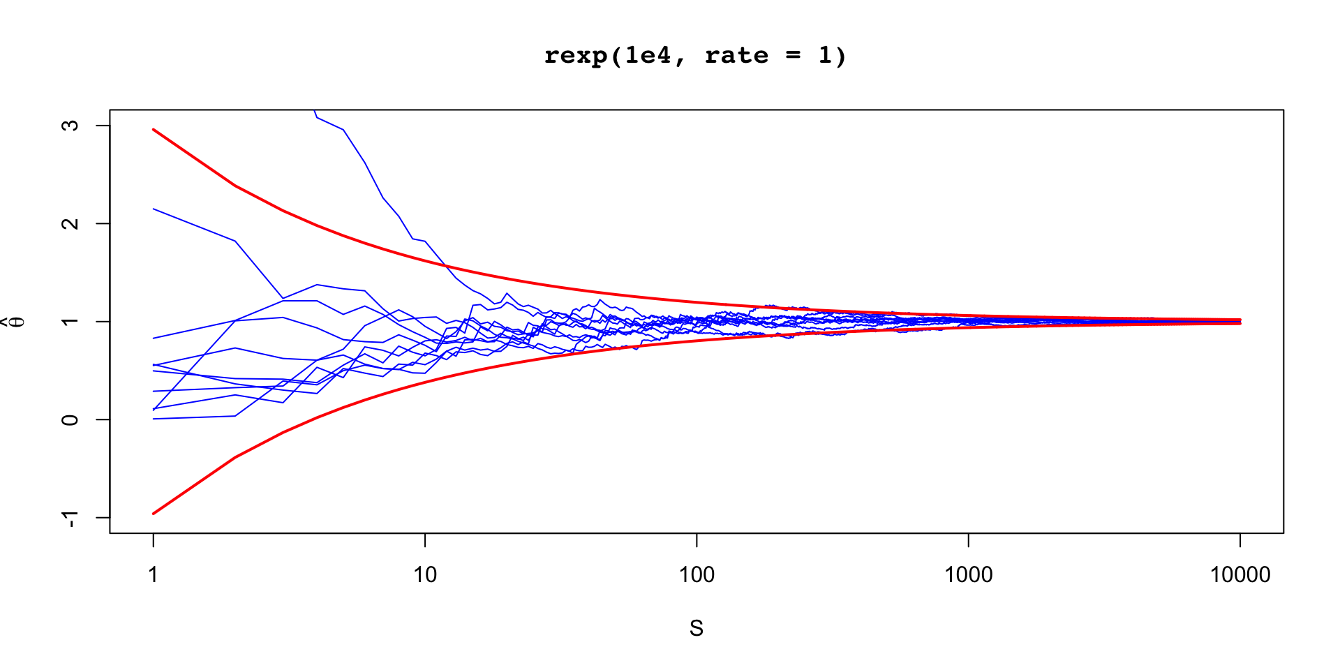
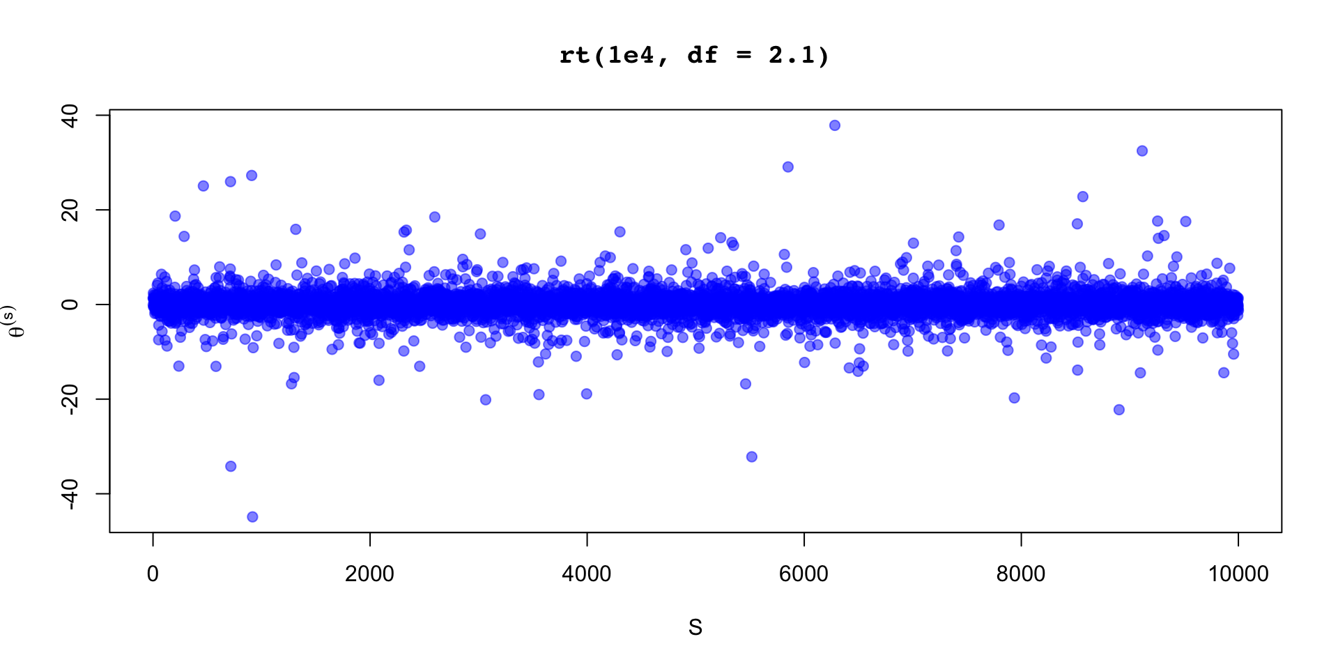
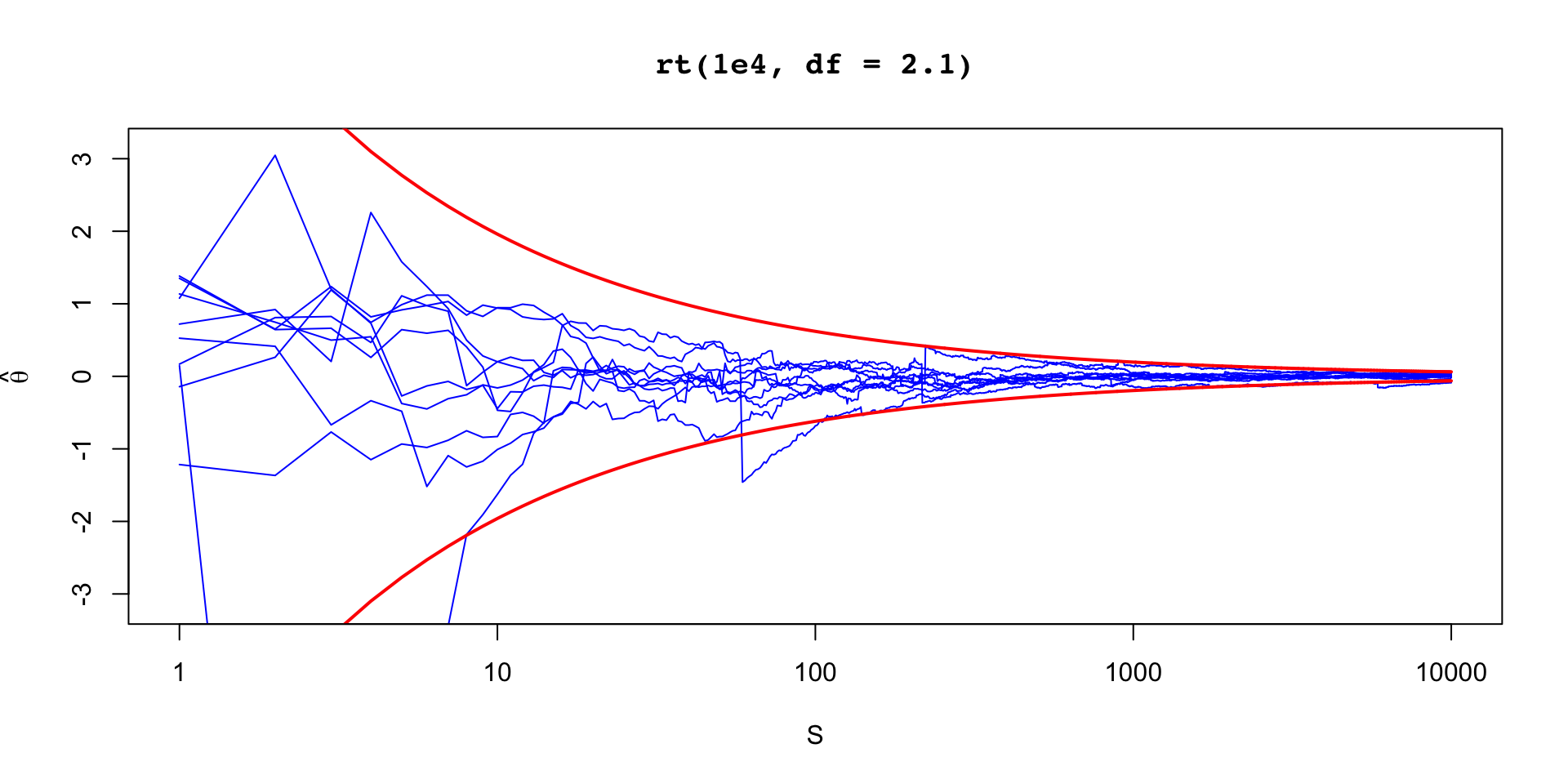
[1] 1
[1] 1.145624e-42
Most models we study in statistical theory courses have closed form expressions for the MLE or the Bayes estimator
On the other hand, the vast majority of statistical models aren’t analytically tractable (e.g. Gamma with unknown shape and scale)
Computation in statistics typically falls into two areas
We’ll focus on stochastic integration and deterministic optimization
\(X_i \sim \text{Gamma}(\alpha, \beta)\)
Find \(\hat{\alpha}_{\text{MLE}}, \hat{\theta}_{\text{MLE}}\)
\[ \begin{aligned} L(\alpha, \theta \mid x) & \propto \prod_{i=1}^n \frac{\beta^\alpha}{\Gamma(\alpha)} x_i^{\alpha - 1} e^{-\beta x_i } \end{aligned} \]
\[ \begin{aligned} \ell(\alpha, \theta \mid x) & = \alpha n \log \beta - n \log \Gamma(\alpha) + (\alpha - 1)\sum_{i=1}^n \log x_i -\beta \sum_{i=1}^n x_i \end{aligned} \]
\[ \begin{aligned} \frac{\alpha}{\beta} - \bar{x} & = 0 \\ \log \beta - \psi(\alpha) + \overline{\log x} & = 0 \end{aligned} \]
Mathematical theorems deal with constructs like \(\R\), but when we’re computing things, we need to contend with limited accuracy
In 64-bit computing, we have 1 bit to determine the sign of the number, 11 bits for the exponent and 52 bits for the mantissa (all of these are in binary): \[ 1.2345 \times 10^5 \]
This would be \(12{,}345\) in floating point
Because of this representation, we can represent numbers near \(0\) very accurately, and we lose accuracy as we increase the magnitude
Smallest number we can represent is about \(2.2\times 10^{-308}\), while closest value to \(1\) is around \(1 \pm 2.2 \times 10^{-16}\)
Because we have limited accuracy, we can’t always compute things the way we write them mathematically
For example, suppose we want to evaluate the likelihood for \(600\) data points we assume come from a normal distribution:
\[ \begin{aligned} y_i \mid \mu & \overset{\text{iid}}{\sim} \text{Normal}(\mu, 1), i = 1, \dots, 600 \\ p(y \mid \mu) & = \prod_{i=1}^{600} \frac{1}{\sqrt{2 \pi}} e^{-\frac{1}{2}(y_i - \mu)^2} \end{aligned} \]
R code, and evaluating \(p(y \mid 0)\) gives:This is called underflow, when the target value exceeds the precision of floating point representation
Intead, we need to compute things on the log scale:
\[ \begin{aligned} \log p(y \mid \mu) & = \sum_{i=1}^{600} -\frac{1}{2} \log(2\pi) -\frac{1}{2}(y_i - \mu)^2 \end{aligned} \]
Suppose you want to compute the log-likelihood in for a mixture model with two components
The likelihood looks like \[ p(y_i \mid \theta) = \phi p(y_i \mid \eta_1) + (1 - \phi) p(y_i \mid \eta_2) \]
We just talked about the importance of keeping things on the log scale so we write: \[ \ell(y_i \mid \eta_1) = \log p(y_i \mid \eta_1) \]
Then our log-likelihood would be
\[ \begin{aligned} \log p(y_i \mid \theta) & = \log( \exp \lp \log(\phi) + \ell(y_i \mid \eta_1) \rp \\ \quad\quad & \exp \lp \log(1 - \phi) + \ell(y_i \mid \eta_2) \rp ) \end{aligned} \]
In Frequentist inference, we (often) need to maximize the likelihood
In Bayesian inference, everything is a posterior expectation:
\[ \ExpA{h(\theta)}{p(\theta \mid y)} = \int h(\theta)p(\theta \mid y)d\theta \]
\[ p(\theta \mid y) = \frac{\textcolor{green}{p(y \mid \theta) p(\theta)}}{\textcolor{red}{\int p(y \mid \theta) p(\theta) d\theta}} \]
We can typically evaluate \(\textcolor{green}{p(y \mid \theta) p(\theta)}\), but \(\textcolor{red}{\int p(y \mid \theta) p(\theta) d\theta}\) is hard to evaluate
Our strategy is to use what we can evaluate \(q(\theta \mid y) = p(y \mid \theta) p(\theta)\) to compute our target expectations
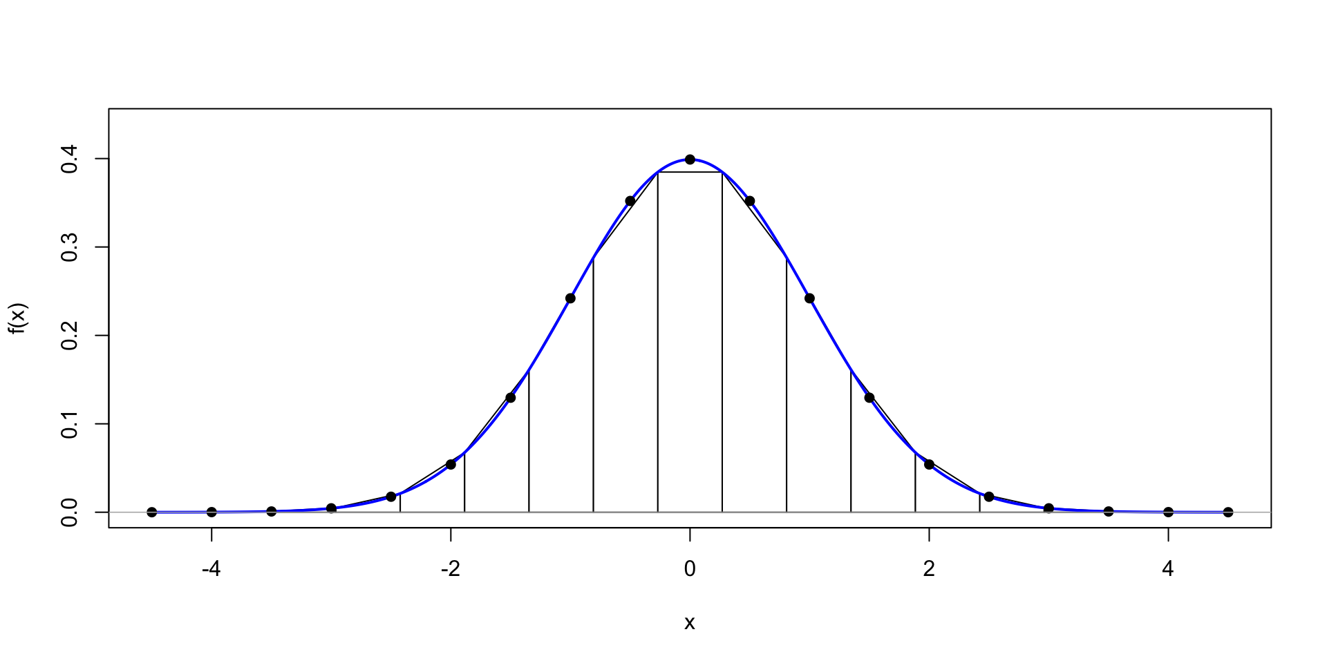
One option is to evaluate \(q(\theta \mid y)\) on a grid of \(\theta^{(s)}\) to get
\[ \ExpA{h(\theta)}{p(\theta \mid y)} \approx \frac{\sum_{s=1}^S h(\theta^{(s)}) q(\theta^{(s)} \mid y)}{\sum_{s=1}^S q(\theta^{(s)} \mid y)} \]
\(\Exp{\theta} = \sum_{s=1}^S \theta^{(s)} w^{(s)}\)
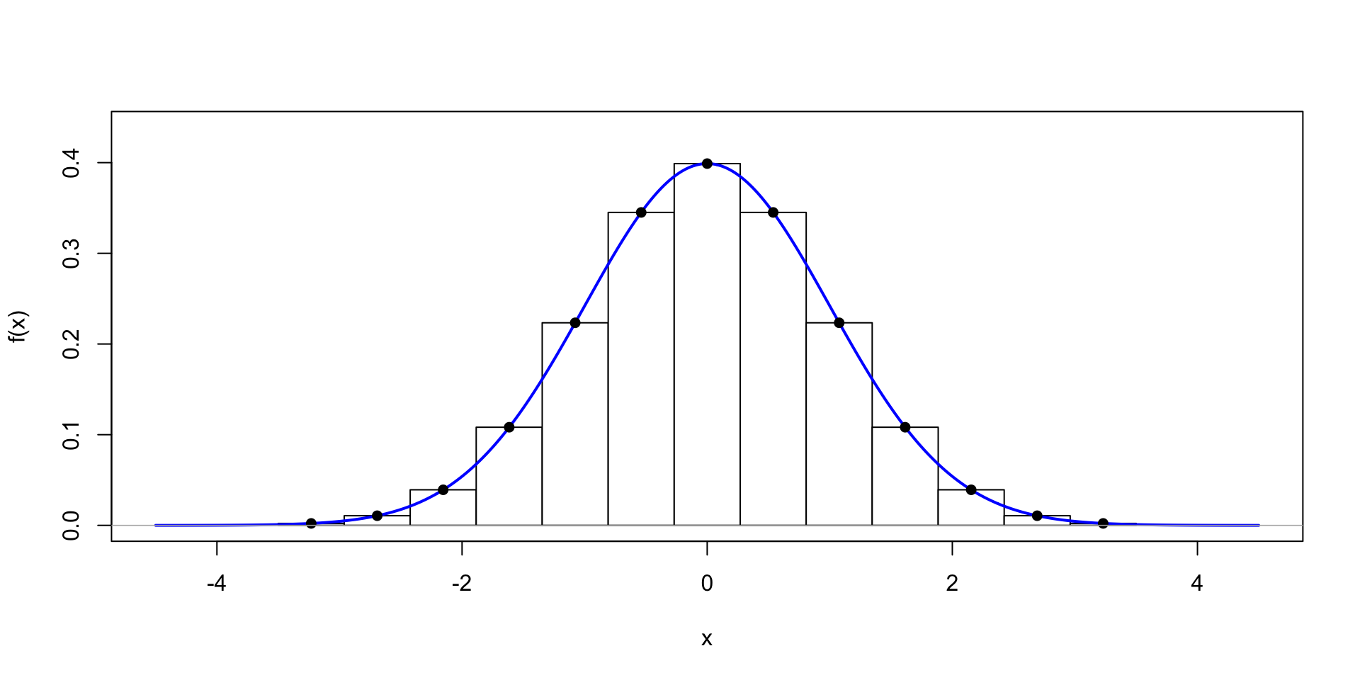

More sophisticated methods are available in R using the integrate function
Evaluations increase exponentially as the dimension of the space increases \(c^d\)
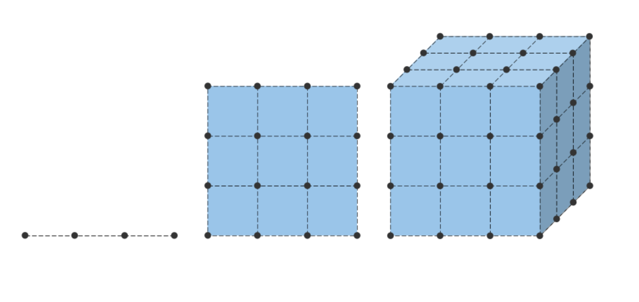
A significant hurdle in grid methods is that you have to define the grid before you know where the mass of the probability distribution
Approximate cost: Suppose we have \(50\) points in each dimension and \(10\) dimensions, this would require \(50^{10} \approx 1e17\) evaluations
Even with a fast computer, this could take years to evaluate
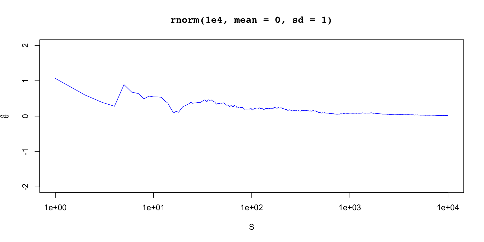
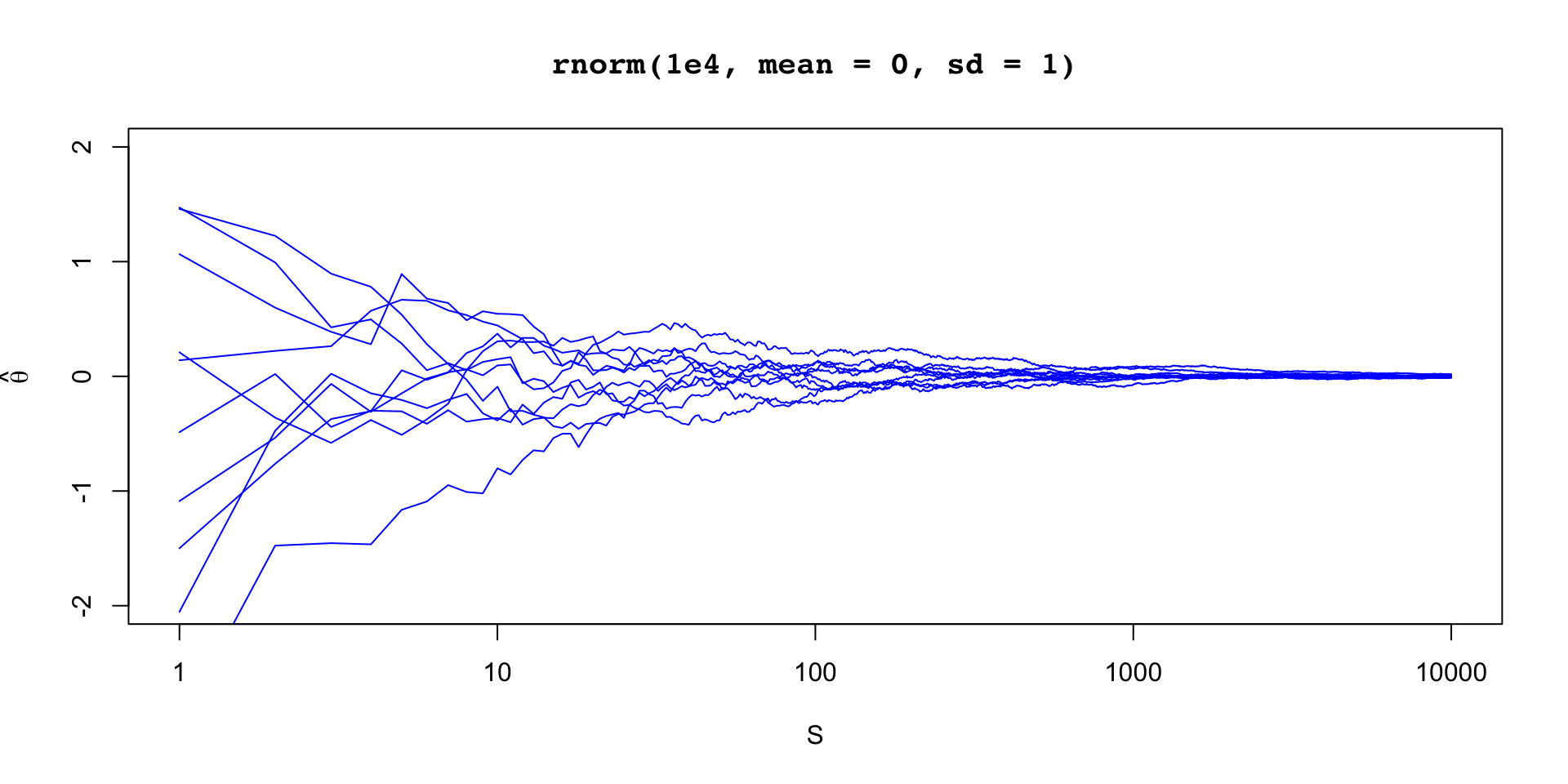
We can take another approach using the laws of large numbers
Say we generate iid draws \(X_i, i = 1, \dots, S\) from some distribution \(F\) and we want to compute \(\Exp{h(X)}\)
If we compute the sample mean
\[ \hat{\mu}_S = \frac{1}{S} \sum_{i=1}^S h(X_i) \]
\[ \lim_{S\to\infty} P(\abs{\hat{\mu}_S - \Exp{h(X)}} < \epsilon) = 1 \]
This says that the probability of the there being a deviation of greater than or equal to \(\epsilon\) is zero in the limit
If \(\Exp{\abs{h(X)}} < \infty\) then we can show that the weak law of large numbers holds


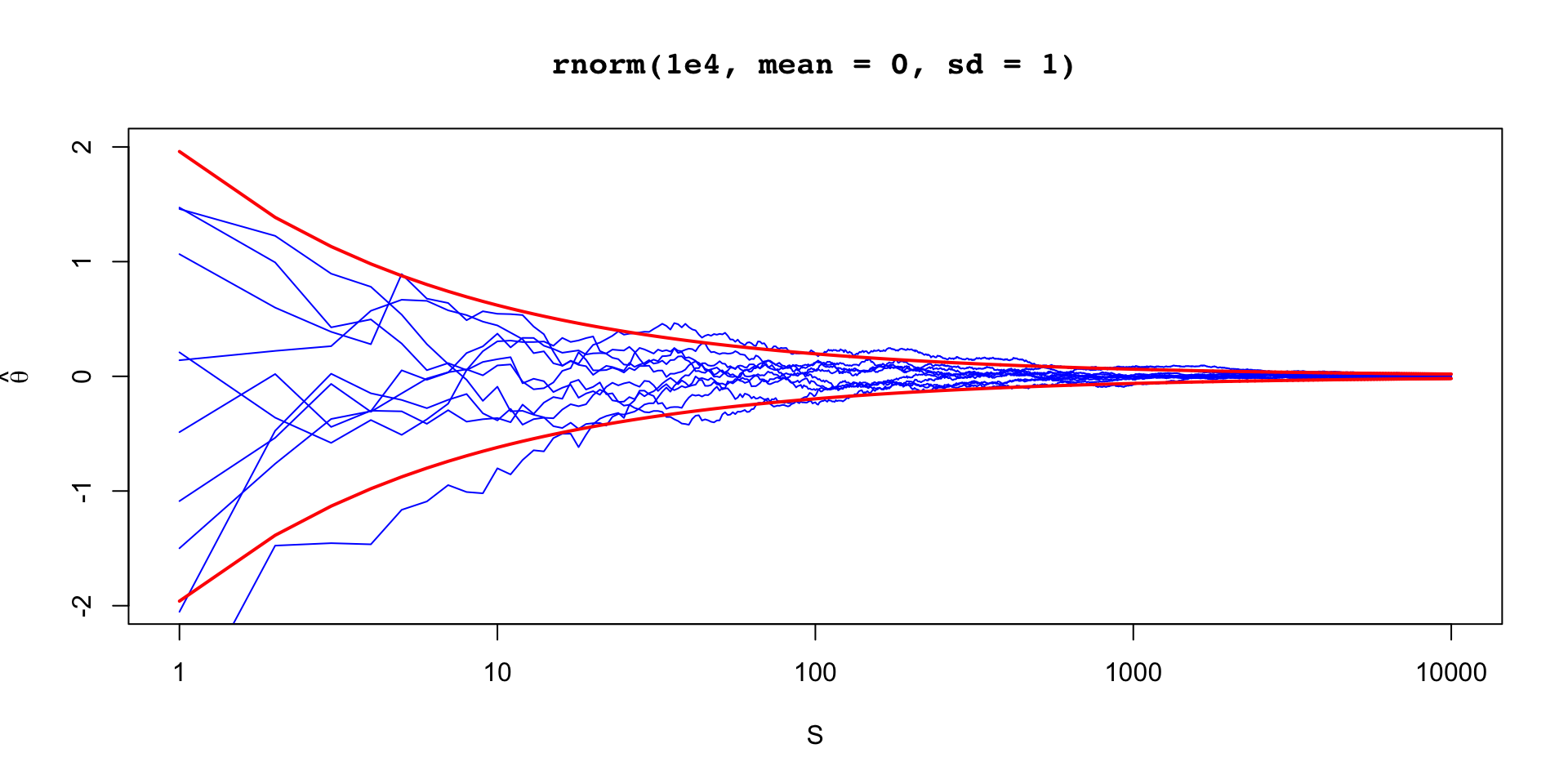
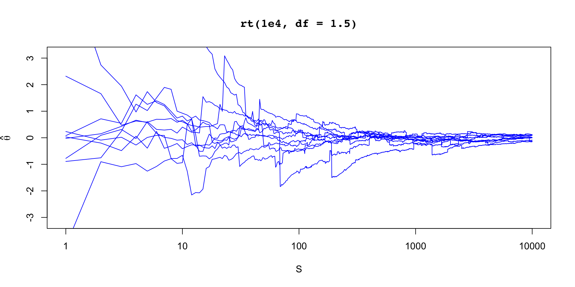
When variance exists, the precision of our estimate is independent of dimension \(\theta\)
\(\text{Var}(\bar{\theta}) = \sigma_\theta^2/S\)
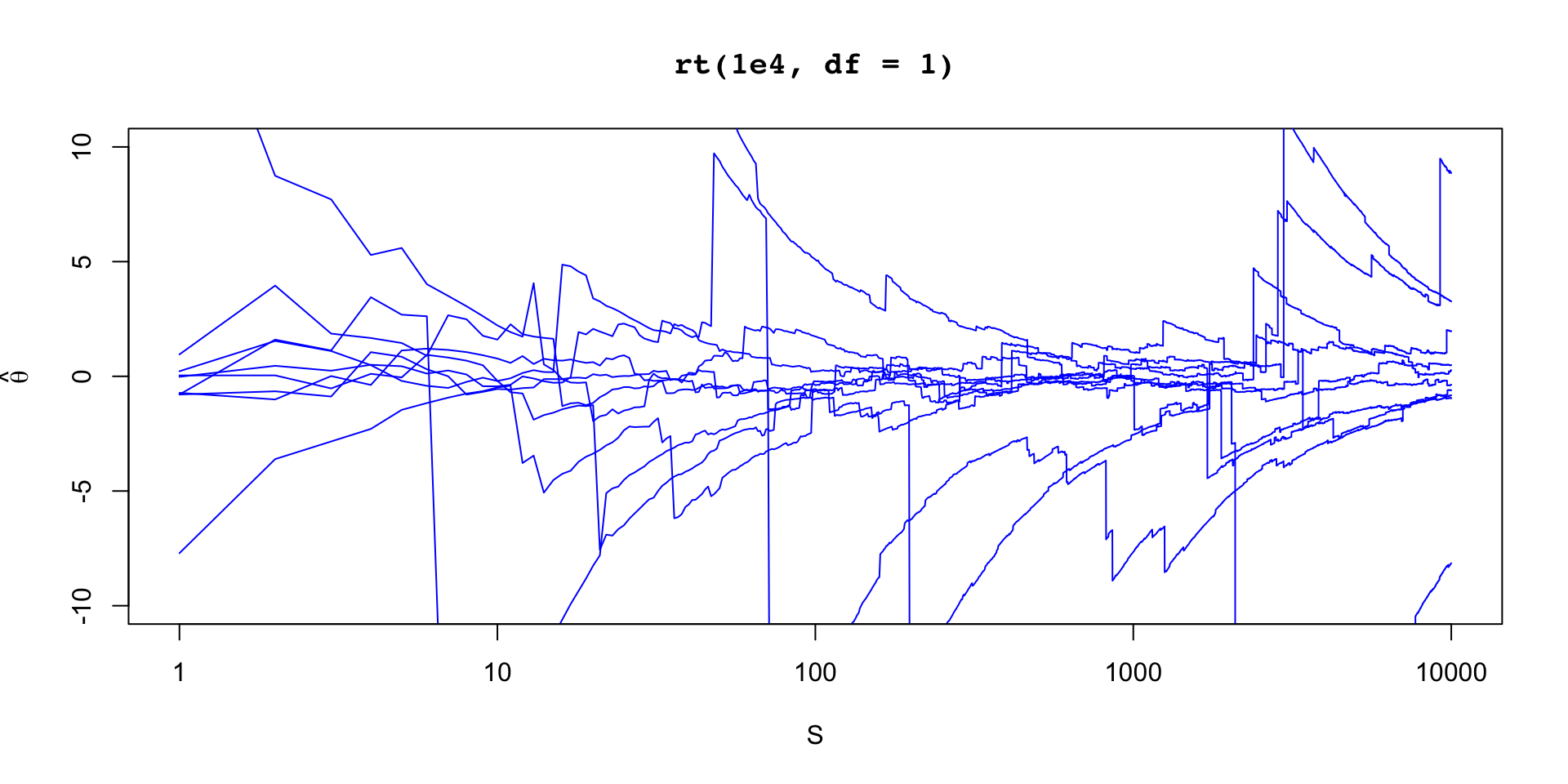
… but need to be sure that variance exists
When variance doesn’t exist but mean does exist there are other limiting distributions, and may still converge to a normal
We have to know how to generate samples from the target distribution
We are bound by the variance of the estimand, \(\sigma_\theta^2\)


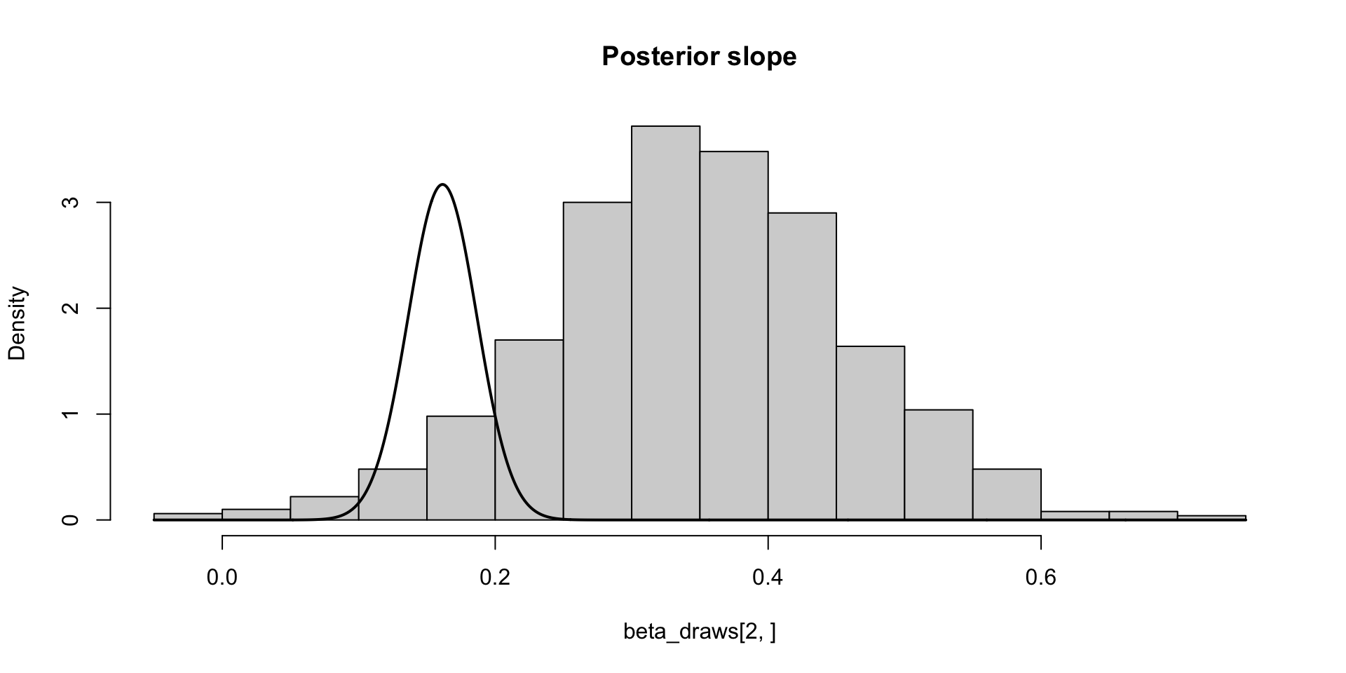
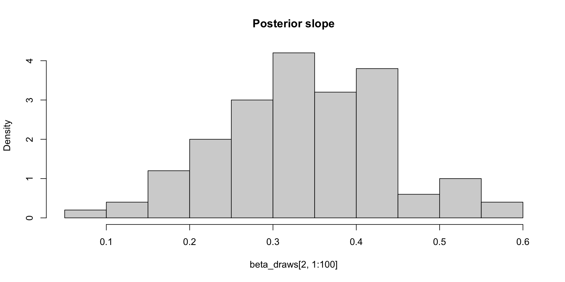
\[ \sigma_\theta \approx 0.12 \implies \text{MCSE}(\hat{\mathbb{E}}[\beta_2 \mid y]) \approx 0.12 / 10 \]
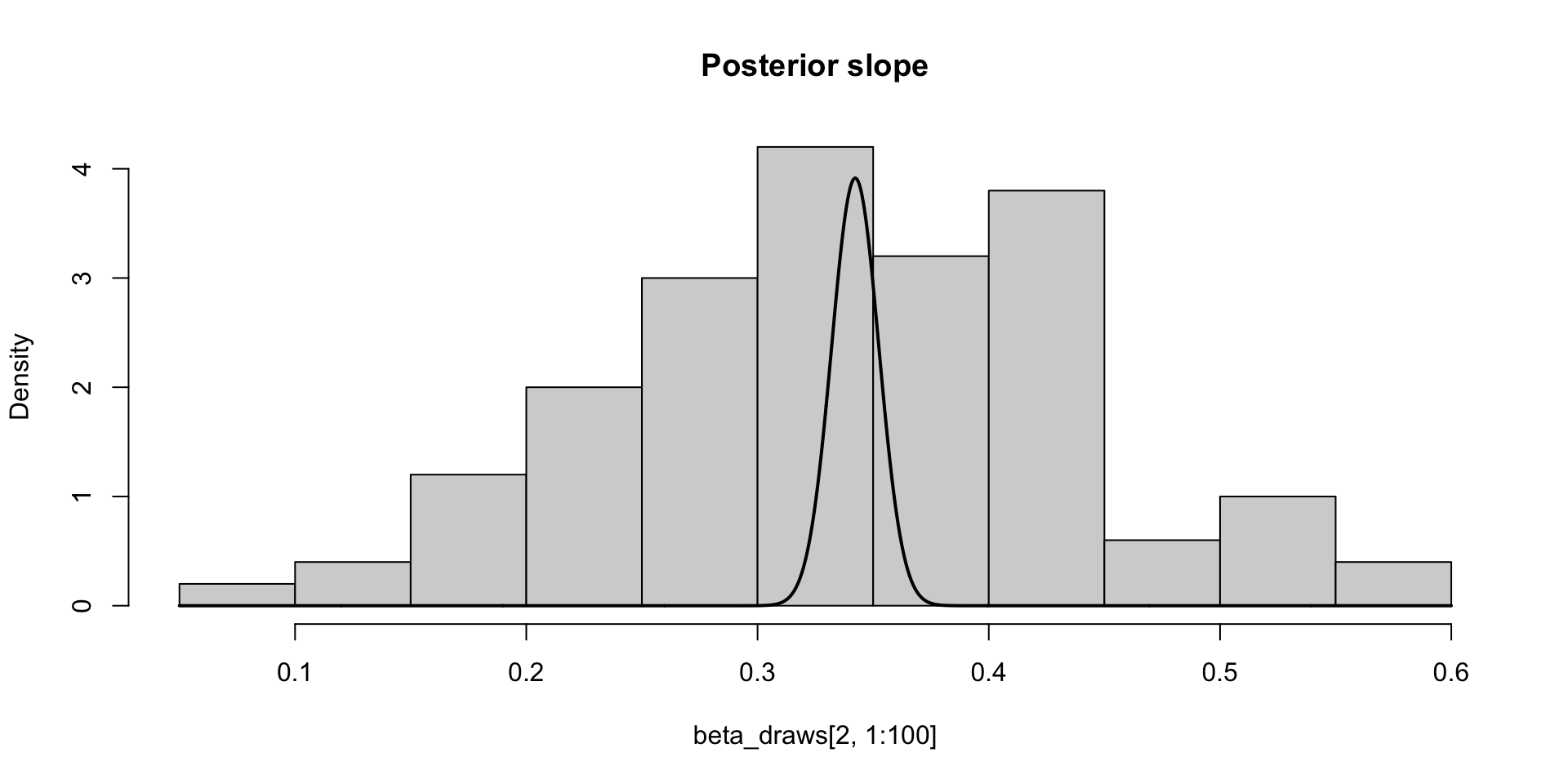
\[ \sigma_\theta \approx 0.10 \implies \text{MCSE}(\hat{\mathbb{E}}[\beta_2 \mid y]) \approx 0.10 / 10 \\ P(\Exp{\beta_2 \mid y} \in (0.32, 0.36)) \approx 0.95 \]
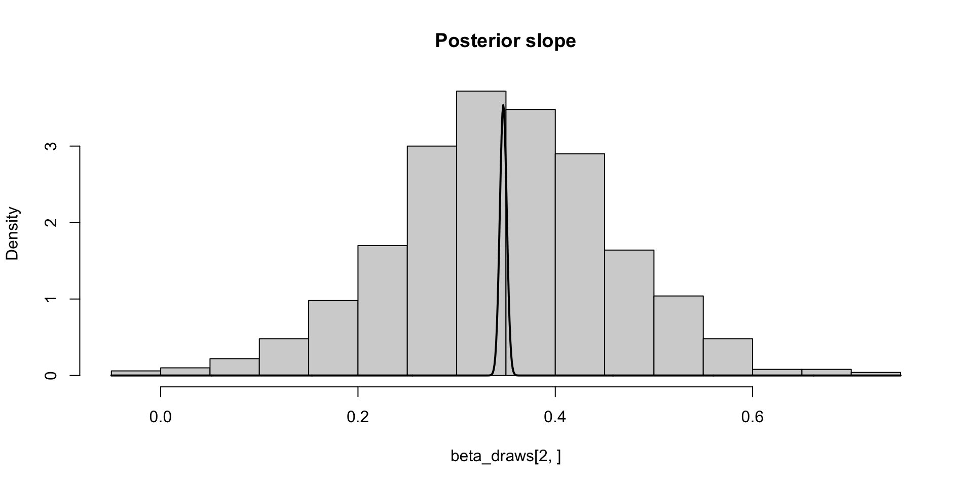
\[ \sigma_\theta \approx 0.12 \implies \text{MCSE}(\hat{\mathbb{E}}[\beta_2 \mid y]) \approx 0.12 / \sqrt{1000} \\ P(\Exp{\beta_2 \mid y} \in (0.35, 0.36)) \approx 0.95 \]
We find the \(p^\mathrm{th}\) quantile by inverting the CDF evaluated at \(p\), \(q = F^{-1}(p)\)
We can find the asymptotic standard error of the \(0.05\) quantile as follows:
Let \(X_s = \ind{\theta^{(s)} \leq a}\)
Let \(\alpha = P(\theta \leq a)\)
Then we know that for i.i.d. \(X_i\) such that \(\Exp{X_i} = \alpha\), \(\bar{X} \overset{\text{d}}{\to} \text{N}(\alpha, \alpha (1 - \alpha)/S)\)
We want to find \(a\) for which \(P(\theta \leq a) = 0.05\)
By Delta method, we know \(g(\bar{X}) \overset{\text{d}}{\to} \text{N}(g(\alpha), \alpha (1 - \alpha) (g'(\alpha))^2 / S)\)
In our case \(g(\alpha) \equiv F^{-1}(\alpha) = a\)
Note:
\[ \begin{aligned} F(F^{-1}(\alpha)) & = \alpha \\ \frac{d}{d\alpha} F(F^{-1}(\alpha)) & = \frac{d}{d\alpha}\alpha \\ f(F^{-1}(\alpha))\frac{d}{d\alpha}F^{-1}(\alpha) & = 1 \\ f(a)\frac{d}{d\alpha}F^{-1}(\alpha) & = 1 \\ \frac{d}{d\alpha}F^{-1}(\alpha) & = 1/f(a) \\ \end{aligned} \]
\[\hat{F}^{-1}(\alpha) \overset{\text{d}}{\to} N(a, \alpha (1 - \alpha) / f(a)^2 S)\]


\[ \text{MCSE}(\hat{F}_{\beta_2 \mid y}^{-1}(0.05)) \approx \sqrt{0.05 \times 0.95} / 10 f(q) \approx 0.03 \\ P(F_{\beta_2 \mid y}^{-1}(0.05) \in (0.11, 0.21)) \approx 0.95 \]
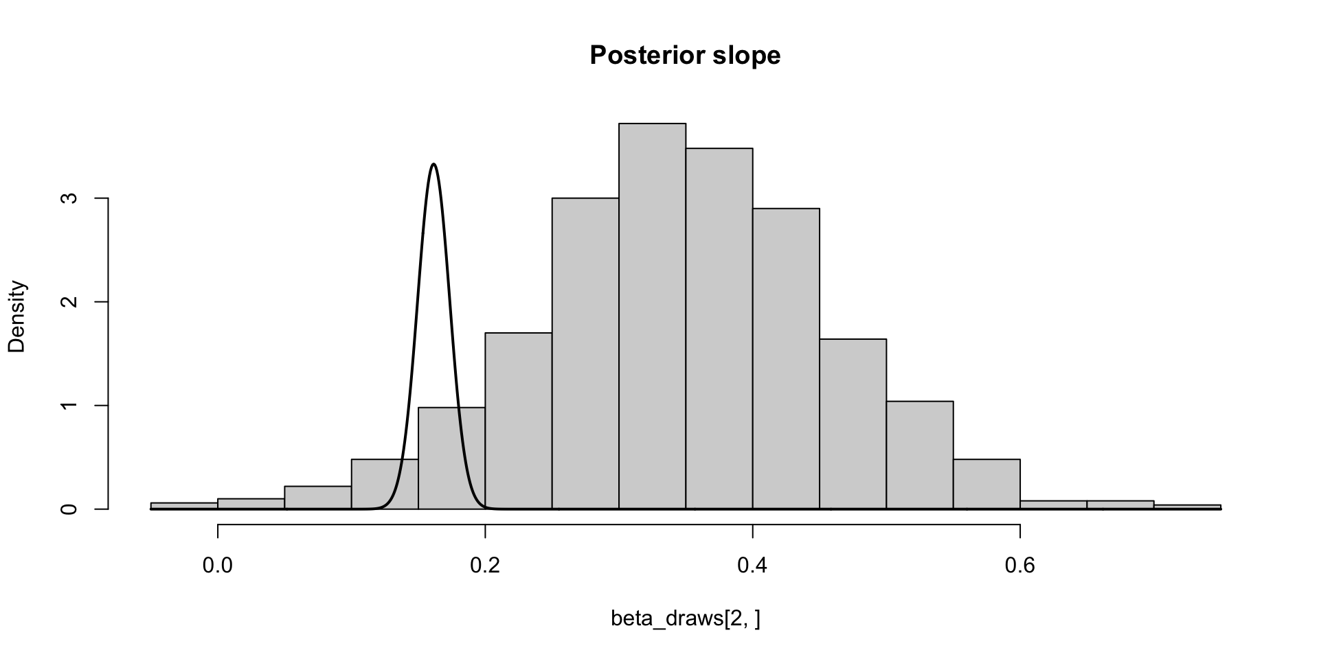
\[ \text{MCSE}(\hat{F}_{\beta_2 \mid y}^{-1}(0.05)) \approx \sqrt{0.05 \times 0.95 / 1000 f(q)} \approx 0.01 \\ P(F_{\beta_2 \mid y}^{-1}(0.05) \in (0.14, 0.18)) \approx 0.95 \]
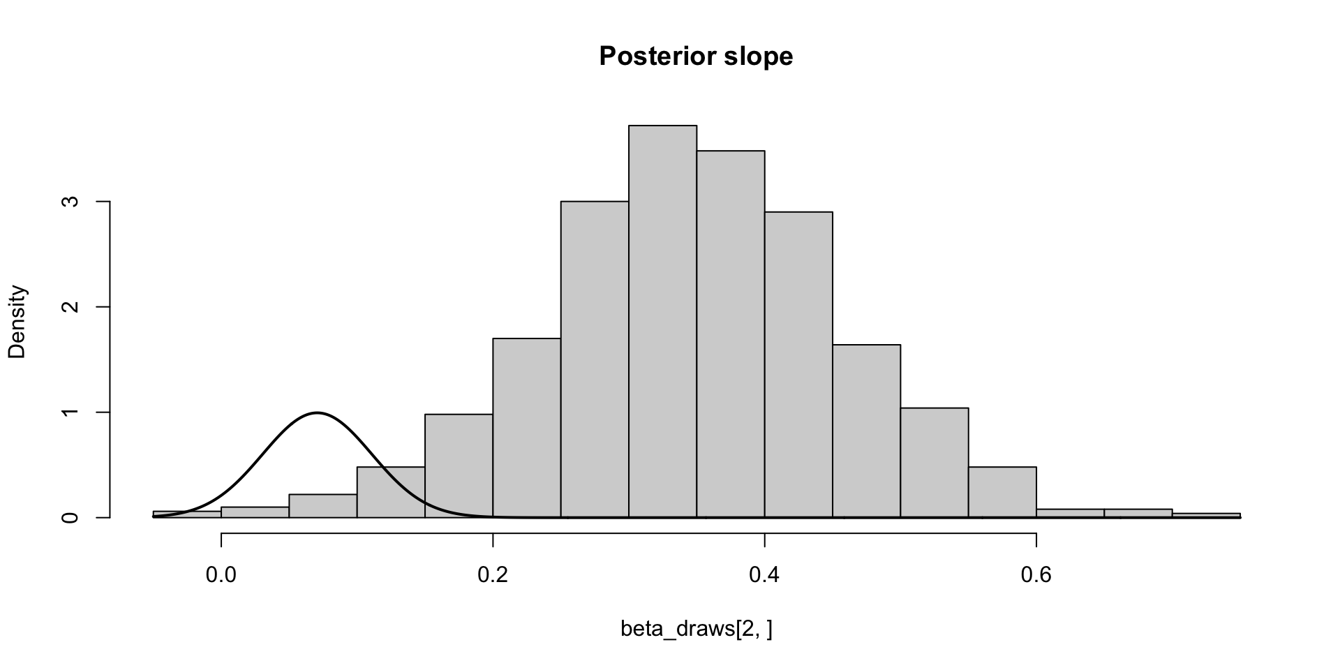
\[ \text{MCSE}(\hat{F}_{\beta_2 \mid y}^{-1}(0.05)) \approx \sqrt{0.01 \times 0.99} / 10 f(q) \approx 0.04\\ P(F_{\beta_2 \mid y}^{-1}(0.01) \in (-0.01, 0.15)) \approx 0.95 \]
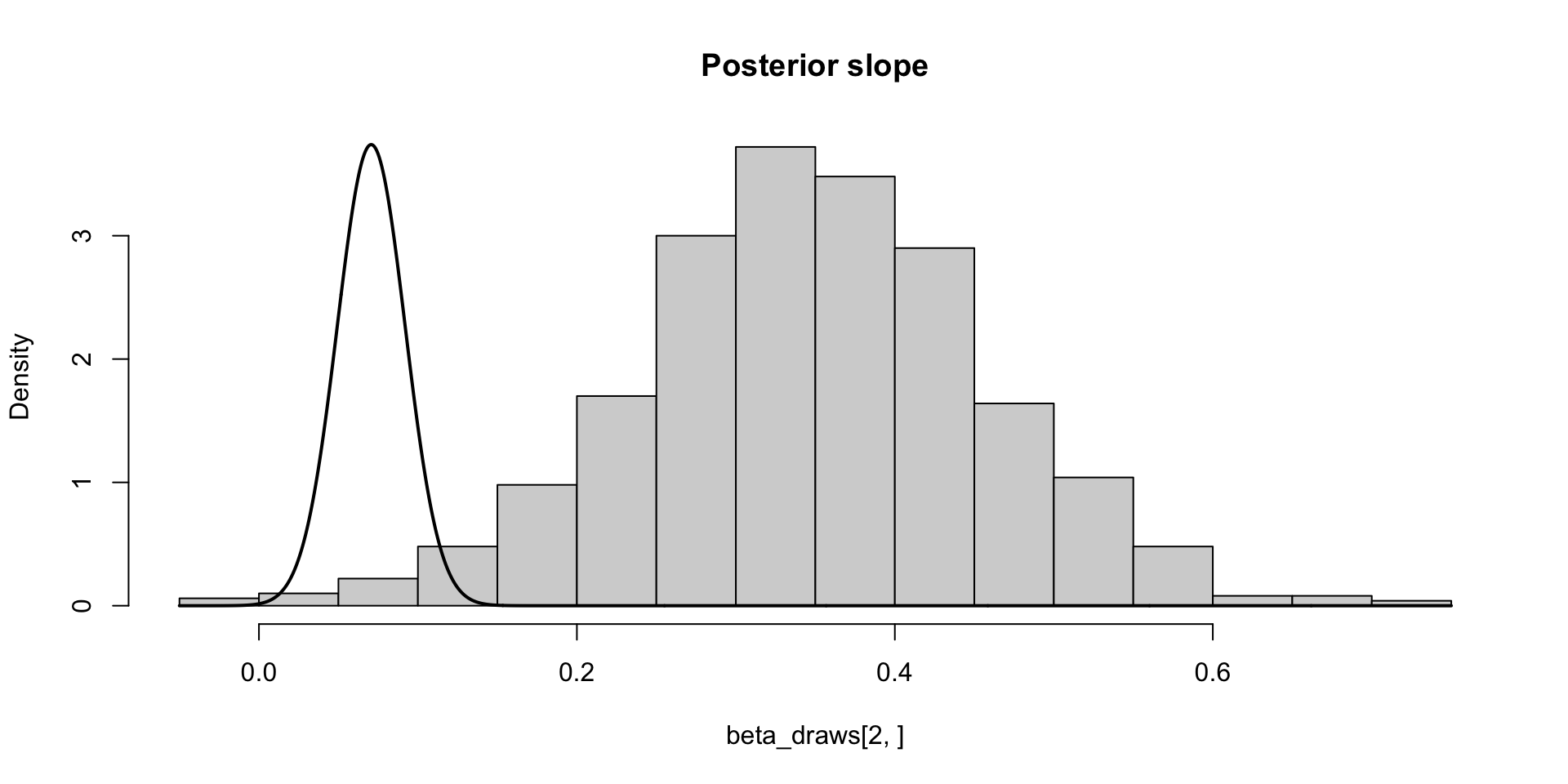
\[ \text{MCSE}(\hat{F}_{\beta_2 \mid y}^{-1}(0.05)) \approx \sqrt{0.01 \times 0.99 / 1000f(q)} \approx 0.02 \\ P(F_{\beta_2 \mid y}^{-1}(0.01) \in (0.03, 0.11)) \approx 0.95 \]
Two types of uncertainty we (typically) need to deal with when doing inference
Statistical uncertainty: quantified by sampling or posterior variance, credible/confidence intervals
Frequentist interpretation: Uncertainty in our estimates driven by the fact that our data is one of many samples of data we could have observed, quantified via variance of sampling distributions, confidence intervals
Bayesian interpretation: Uncertainty in our estimates driven by the fact that our given data set could have been generated by one of many parameter values, quantified via posterior variance, and credible intervals (aka posterior intervals)
Monte Carlo uncertainty: Uncertainty given by the fact that we have finite number of samples from a distribution to compute a quantity of interest
Both types of uncertainty exist when we do Bayesian statistics
Monte Carlo uncertainty enters into how we quantify posterior uncertainty when we have samples from the posterior
We quantify Monte Carlo uncertainty with the CLT
To easily apply the CLT, we need to know if first and second moments exist[^1] [^1] We don’t need a mean or variance for the CLT to hold, but if the first two moments exist we can apply the CLT
If we have a set samples \(\{\theta^{(s)}, s = 1, \dots, S\}\) from \(p(\theta \mid y)\), is there a way to determine if \(\Exp{\theta^k \mid y}\) exists?
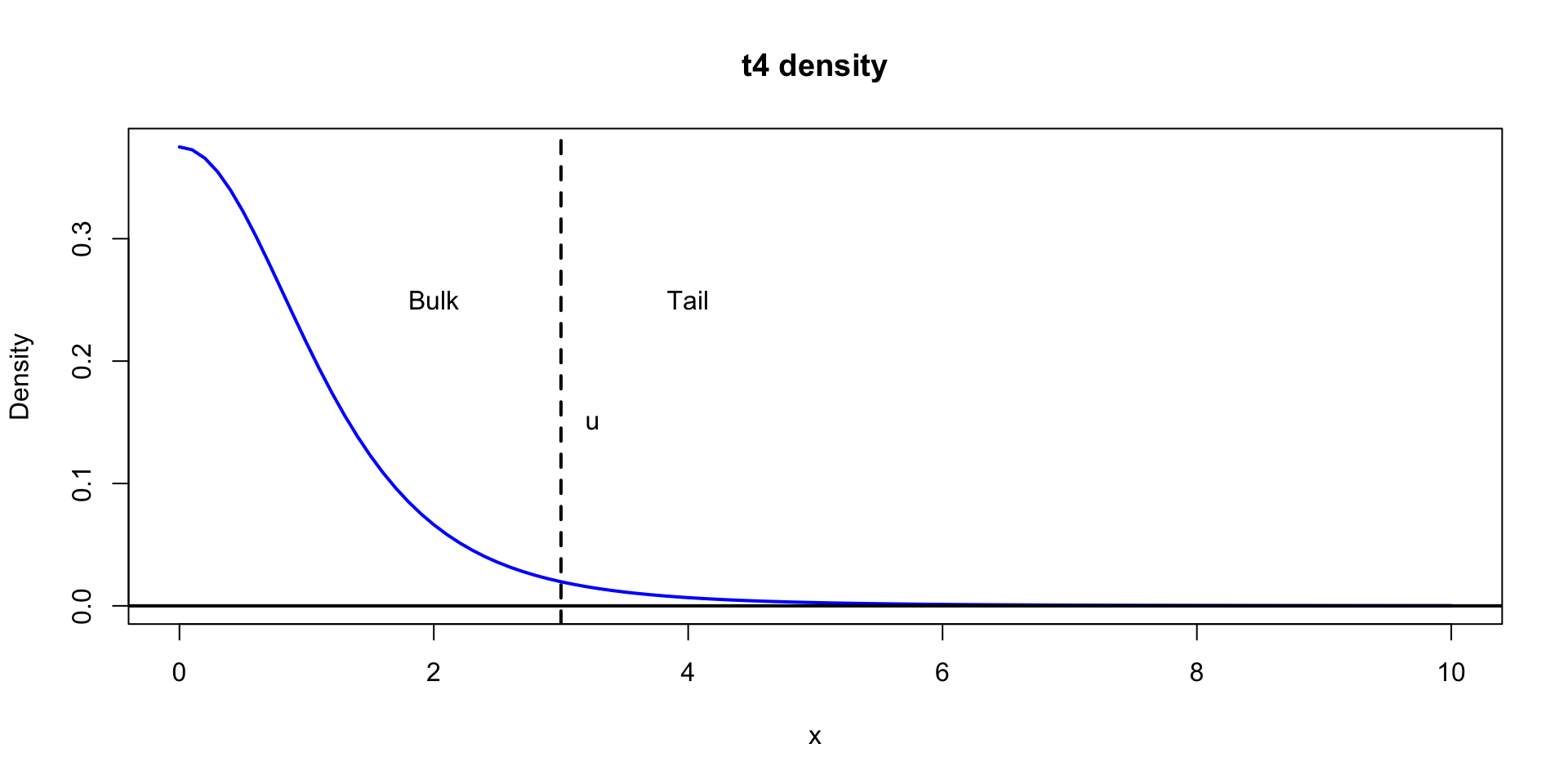
The answer lies in characterizing the tails of the distribution of \(\theta \mid y\)
We know that \(\Exp{X} = \int x f(x) dx\)
Let’s just focus on \(X > 0\). We can write, for large, finite \(K\)
\[ \int_0^\infty x f(x) = \int_{x < K} x f(x) dx + \int_{K}^{\infty} x f(x) dx \]
\[ \int_0^\infty x f(x) \leq K P(X < K) + \int_{K}^{\infty} x^{-(1 + \delta)} dx < \infty \]
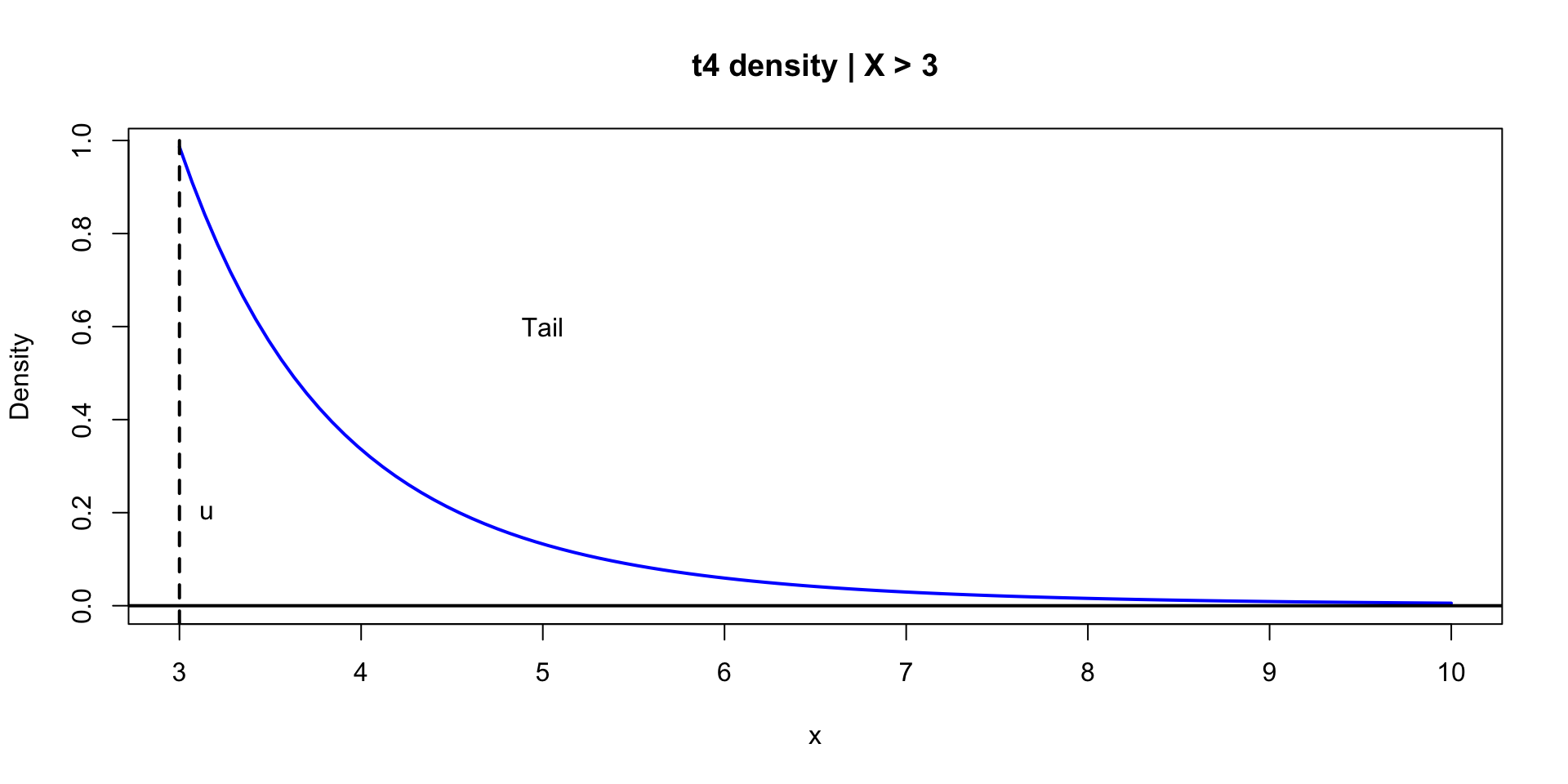
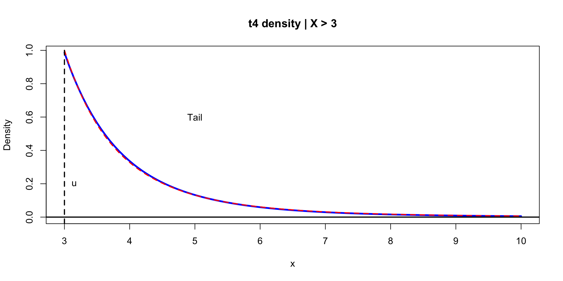
\[ p(y \mid u, \sigma, k) = \begin{cases} \frac{1}{\sigma}(1 + k \lp \frac{y - u}{\sigma} \rp)^{-(1 + 1/k)}, & k \neq 0 \\ \frac{1}{\sigma}\exp\lp \frac{y - u}{\sigma} \rp), & k = 0 \end{cases} \]
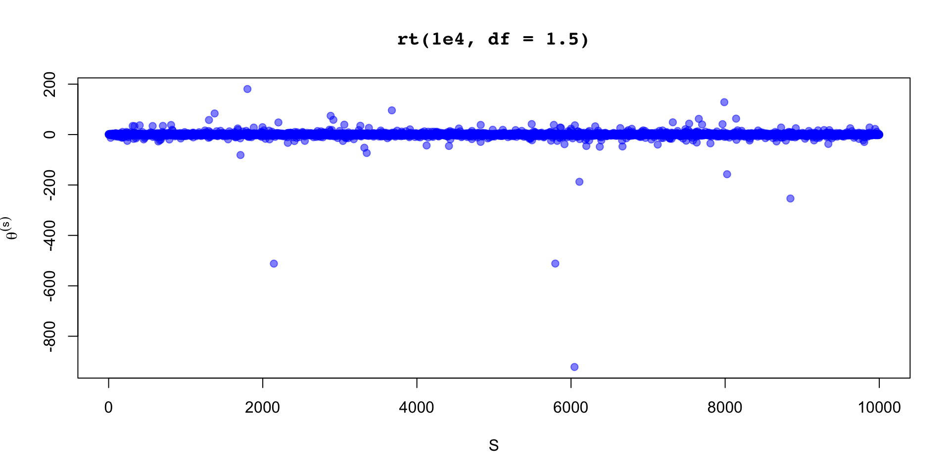
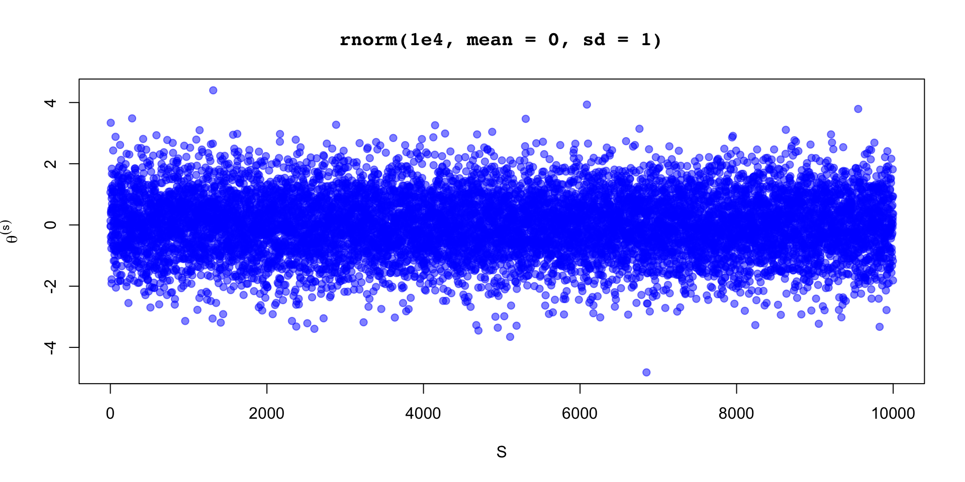
\(\theta \sim \text{Normal}(0,1)\)
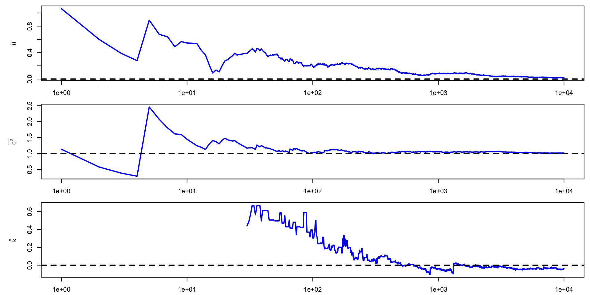
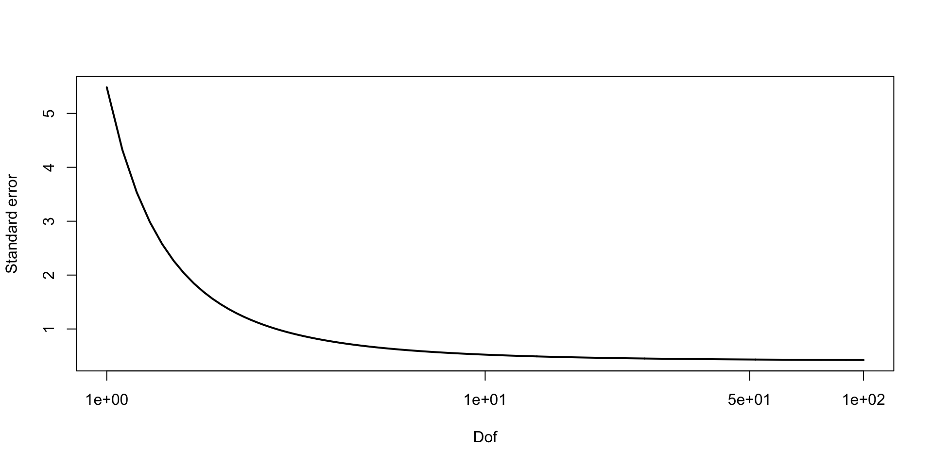
\(\theta \sim \text{t}(4, 0,1)\)
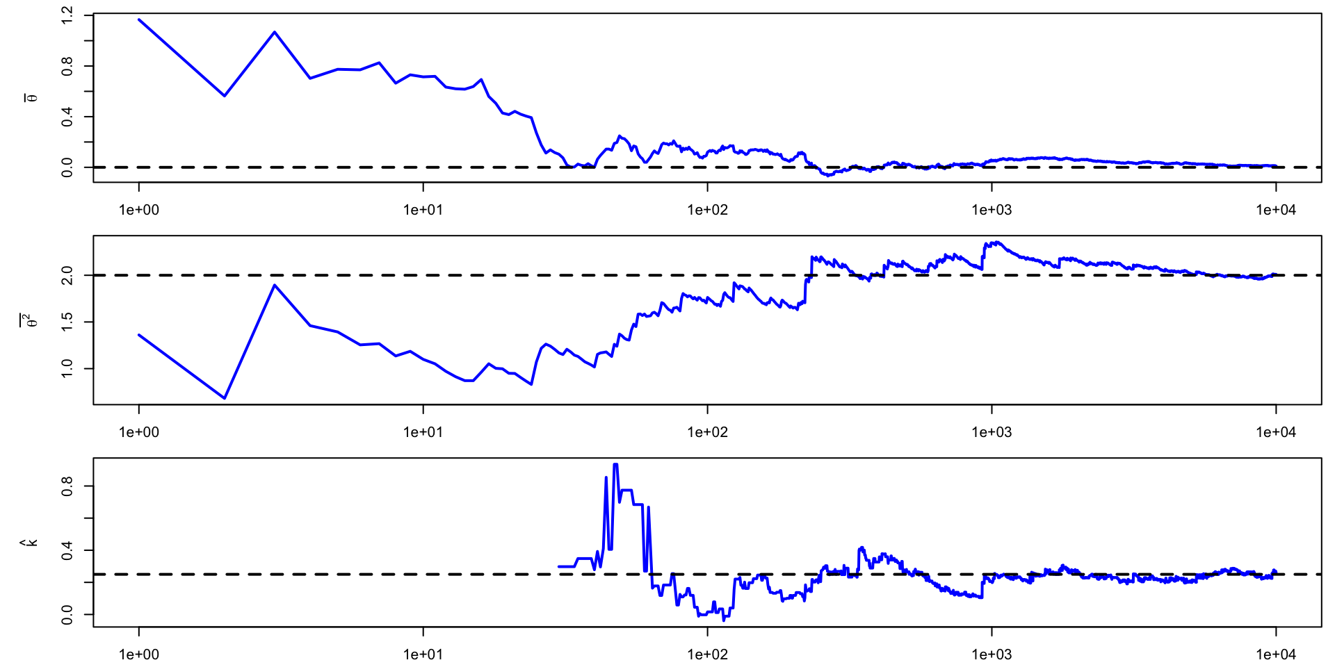
\(\theta \sim \text{t}(2, 0,1)\)
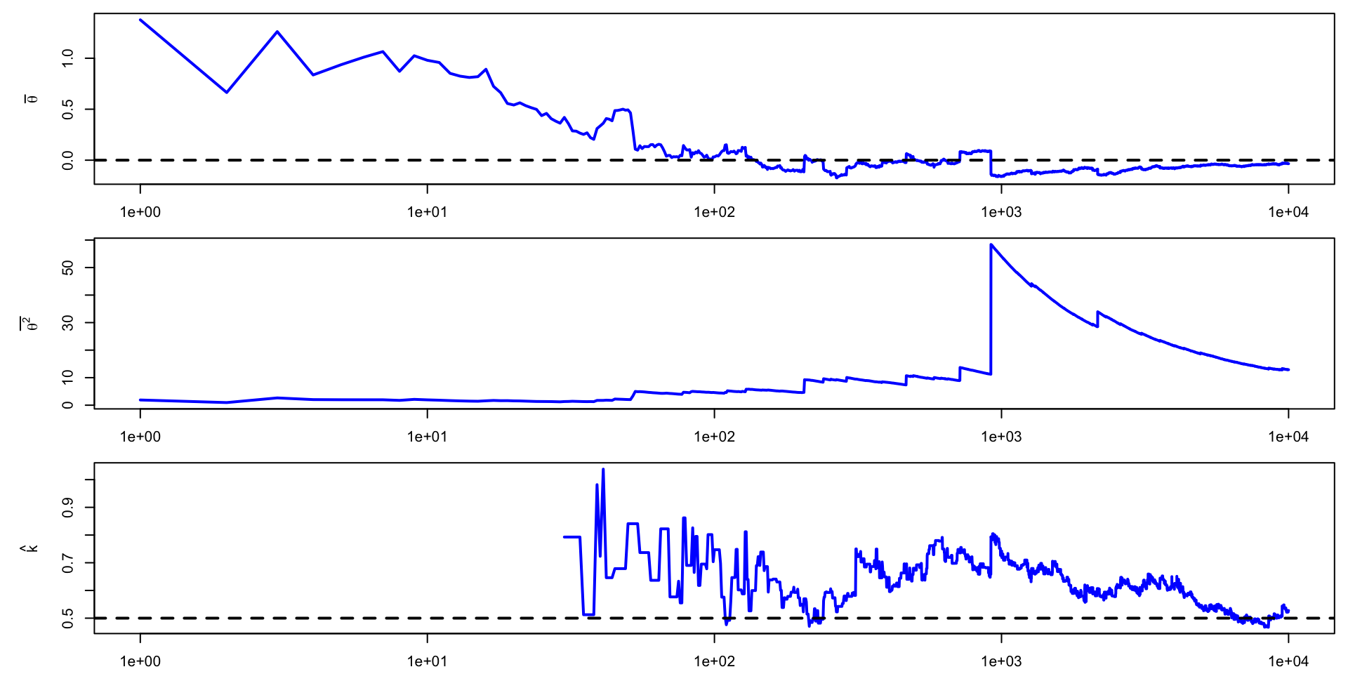
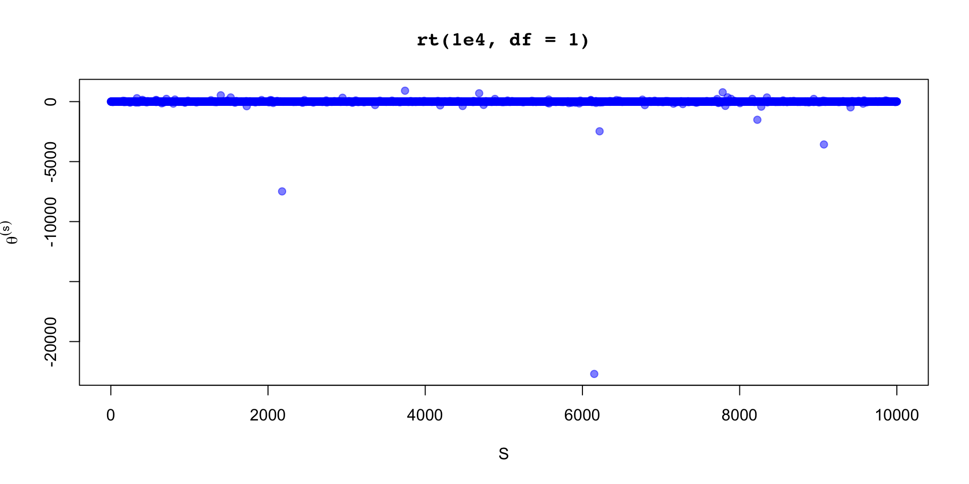
\(\theta \sim \text{t}(1, 0,1)\)
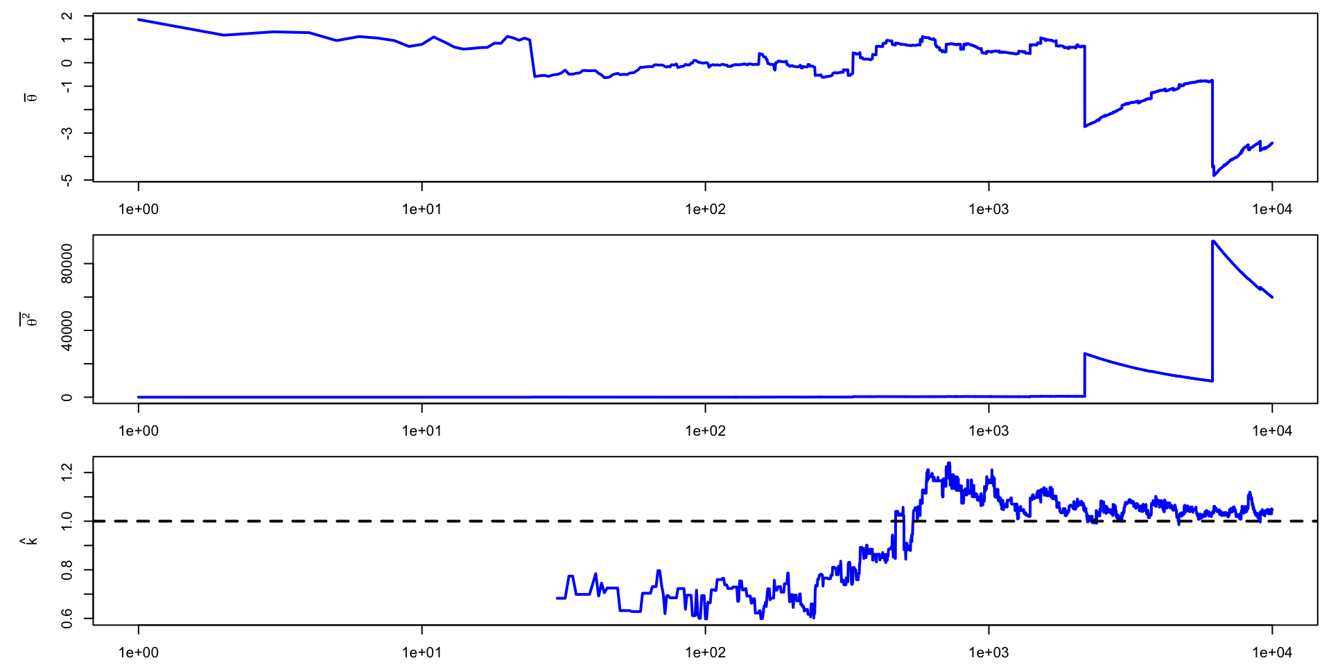
posterior parckage# A tibble: 4 × 5
variable mean sd mcse_mean pareto_khat
<chr> <dbl> <dbl> <dbl> <dbl>
1 norm 0.014 1.0 0.010 -0.089
2 rt4 0.0043 1.4 0.014 0.30
3 rt2 0.00038 3.0 0.030 0.50
4 rt1 -0.37 104. 1.0 0.94
If \(\hat{k}\) is large, use a quantile to summarize the posterior instead of a moment
There is, of course, variance in \(\hat{k}\) estimation because of finite sample size
For \(\hat{k} < 0.7\) one can use smoothing to increase the efficiency of the mean estimate
For more info see Vehtari et al. (2024)