Lecture 14: Cox model continued

1 Score function of the Cox model

Given that we’ll use maximum likelihood to fit the Cox model, the score equations for the Cox model will be of importance to us. As shown in the previous section, the partial likelihood is: \[\begin{align} PL(\boldsymbol{\beta}) & = \prod_{i=1}^n \left(\frac{\exp(\mathbf{z}_i^T \boldsymbol{\beta})}{\sum_{j \in R(t_i)} \exp(\mathbf{z}_j^T \boldsymbol{\beta})}\right)^{\delta_i} \end{align}\] The log-partial likelihood is thus \[\begin{align} \log PL(\boldsymbol{\beta})=p\ell(\boldsymbol{\beta}) & = \sum_{i=1}^n \delta_i \left(\mathbf{z}_i^T \boldsymbol{\beta} - \log \left(\sum_{j \in R(t_i)} \exp(\mathbf{z}_j^T \boldsymbol{\beta})\right)\right) \end{align}\] The gradient of this function with respect to the parameter vector \(\boldsymbol{\beta}\) is \[\begin{align} p\ell_\boldsymbol{\beta}(\boldsymbol{\beta}) & = \sum_{i=1}^n \delta_i \left(\mathbf{z}_i - \frac{\sum_{j \in R(t_i)} \mathbf{z}_j \exp(\mathbf{z}_j^T \boldsymbol{\beta})}{ \sum_{j \in R(t_i)} \exp(\mathbf{z}_j^T \boldsymbol{\beta})}\right) \end{align} \tag{1}\] This can be seen to be the difference between the covariate value for individual \(i\) who fails at time \(t_i\) and the weighted average covariate value for individuals in the risk set at \(t_i\).

2 Observed Fisher Information matrix for the Cox model

In order to define the infomration matrix, it’ll help to define some notation for some of the expressions appearing in Equation 1. Let \[p_j(\beta, t_i) = \frac{\exp(\mathbf{z}_j^T \boldsymbol{\beta})}{ \sum_{k \in R(t_i)} \exp(\mathbf{z}_k^T \boldsymbol{\beta})}\] and let \[\ExpA{z \mid \beta}{R(t_i)} = \sum_{j \in R(t_i)} \mathbf{z}_j p_j(\beta, t_i)\] \[\begin{align} p\ell_{\boldsymbol{\beta}\boldsymbol{\beta}}(\boldsymbol{\beta}) & = -\sum_{i=1}^n \delta_i \sum_{j \in R(t_i)} \left(\mathbf{z}_j - \ExpA{z \mid \beta}{R(t_i)}\right)\left(\mathbf{z}_j - \ExpA{z \mid \beta}{R(t_i)}\right)^T p_j(\beta, t_i) \end{align}\] The observed Fisher information is then \(-p\ell_{\boldsymbol{\beta}\boldsymbol{\beta}}(\hat{\boldsymbol{\beta}})\), or \[\sum_{i=1}^n \delta_i \sum_{j \in R(t_i)} \left(\mathbf{z}_j - \ExpA{z \mid \hat{\beta}}{R(t_i)}\right)\left(\mathbf{z}_j - \ExpA{z \mid \hat{\beta}}{R(t_i)}\right)^T p_j(\hat{\beta}, t_i)\]

Example 1. Simple two-group Cox regression example Let’s assume that we observe failure time data from two groups, \(1\) and \(2\), that contain no tied event times. The observed data is \(\{(t_i, \delta_i, z_i), i = 1, \dots, n\}\). Each observation \(i\) is paired with a scalar value \(z_i\) taking the value \(0\) when \(i\) is in group 1, and \(1\) otherwise. The hazard model takes the form: \[\lambda_i(t) = \lambda_0(t) \exp(\beta z_i).\] with \(\lambda_0(t)\) left unspecified.

The partial likelihood for \(\beta\) is \[\begin{align} \prod_{i=1}^n \left(\frac{\exp(\beta z_i)}{\sum_{k \in R(t_i)} \exp(\beta z_k)}\right)^{\delta_i} \end{align} \tag{2}\] Equation 2 simplifies if we create an alternative dataset by generating \(\{\tau_j = t_i \mid \delta_i = 1\}\), and \(\{(\tau_j, \delta_{2j}), j = 1, \dots r = \sum_i \delta_i\}\) the times of observed failures: \[\begin{align} \label{eq:simplified-cox-model} \prod_{j=1}^r \frac{\exp(\beta \delta_{2j})}{\sum_{k \in R(\tau_j)} \exp(\beta z_k)} \end{align}\] Let’s write out the log-likelihood and the score equation for \(\beta\): \[\begin{align} \label{eq:log-lik-cox} \sum_{j=1}^r \beta \delta_{2j} - \sum_{j=1}^r \log\left(\sum_{k \in R(\tau_j)} \exp(\beta z_k)\right) \end{align}\] This can again be simplified if we keep track of the number of individuals at risk in each group. Let these variables be, as before, denoted \(\widebar{Y}_{1}(\tau_j), \widebar{Y}_{2}(\tau_j)\). As a reminder, we define these variables as: \[\begin{align} \widebar{Y}_{1}(\tau_j) & = \sum_{i=1}^n (1 - z_i) \mathbbm{1}\left(t_i \geq \tau_j\right) \\ \widebar{Y}_{2}(\tau_j) & = \sum_{i=1}^n z_i \mathbbm{1}\left(t_i \geq \tau_j\right) \end{align}\] Because \(z_k = 0\) for all \(\widebar{Y}_{1}(\tau_j)\) we get \[\begin{align} \sum_{j=1}^r \beta \delta_{2j} - \sum_{j=1}^r \log\left(\widebar{Y}_{1}(\tau_j) + \widebar{Y}_{2}(\tau_j)e^\beta\right) \end{align}\] One more simplification is that \(\sum_{j=1}^r \delta_{2j} = \sum_{i=1}^n \delta_i z_i\), which we’ll call \(r_{2}\), or the total failures in group \(2\). \[\begin{align} r_2 \beta - \sum_{j=1}^r \log\left(\widebar{Y}_{1}(\tau_j) + \widebar{Y}_{2}(\tau_j)e^\beta\right) \end{align}\] Taking the gradient with respect to \(\beta\) gives: \[\begin{align} r_2 - \sum_{j=1}^r \frac{\widebar{Y}_{2}(\tau_j)e^\beta}{\widebar{Y}_{1}(\tau_j) + \widebar{Y}_{2}(\tau_j)e^\beta} \end{align}\] Setting this equation equal to zero leads to an equation we cannot explicitly solve in terms of \(\beta\): \[\begin{align} \sum_{j=1}^r \frac{\widebar{Y}_{2}(\tau_j)e^\beta}{\widebar{Y}_{1}(\tau_j) + \widebar{Y}_{2}(\tau_j)e^\beta} = r_2 \end{align}\]

An alternative is to use the score test. Here is the benefit of the score test in examples like these, where we don’t have to maximize the log-likelihood under the alternative in order to test the hypothesis that the rates of failure are different between the two groups. Take a look at the lecture on the score test to remind yourself about what the score test entails.

Here is the score equation for \(\beta\) \[\begin{align} \sum_{j=1}^r \left(\delta_{2j} - \frac{\widebar{Y}_{2}(\tau_j)e^\beta}{\widebar{Y}_{1}(\tau_j) + \widebar{Y}_{2}(\tau_j)e^\beta}\right) \end{align}\] The second derivative of the log-likelihood with respect to \(\beta\) is \[\begin{align} -\sum_{j=1}^r \frac{\widebar{Y}_{1}(\tau_j) \widebar{Y}_{2}(\tau_j)e^\beta}{(\widebar{Y}_{1}(\tau_j) + \widebar{Y}_{2}(\tau_j)e^\beta)^2} \end{align}\] The score test statistic is formed by evaluating the score and the observed information at \(\beta=0\): \[\begin{align} \begin{split} \ell_\beta(0) & = \sum_{j=1}^r \left(\delta_{2j} - \frac{\widebar{Y}_{2}(\tau_j)}{\widebar{Y}_{1}(\tau_j) + \widebar{Y}_{2}(\tau_j)}\right)\\ -\ell_\beta(0) & = \sum_{j=1}^r \frac{\widebar{Y}_{1}(\tau_j) \widebar{Y}_{2}(\tau_j)}{(\widebar{Y}_{1}(\tau_j) + \widebar{Y}_{2}(\tau_j))^2} \end{split} \end{align} \tag{3}\] These are exactly the numerator and the denominator of the log-rank test statistic when there are no ties present. Remember, the log-rank test, using data collected through time point \(\tau\) is \[\frac{Z_j(\tau)}{\sqrt{\text{Var}(Z_j(\tau))}}\] With expressions for numerator and denominator below: \[\begin{align} Z_j(\tau) & = \sum_{i=1 \mid t_i \leq \tau}^{n_1 + n_2} W(t_i) \left(d_{ij} - d_i\frac{\widebar{Y}_j(t_i)}{\widebar{Y}(t_i)}\right)\\ \Var{Z_j(\tau)} & =\sum_{i} W(t_i)^2 \left(d_i\frac{\widebar{Y}_j(t_i)}{\widebar{Y}(t_i)} \left(1 - \frac{\widebar{Y}_j(t_i)}{\widebar{Y}(t_i)}\right)\frac{\widebar{Y}(t_i) - d_i}{\widebar{Y}(t_i) - 1 }\right) \end{align}\] In our case here, \(d_i\) is always equal to \(1\) because we have no ties. With two groups \(1 - \frac{\widebar{Y}_j(t_i)}{\widebar{Y}(t_i)}\) is \(\frac{\widebar{Y}_1(t_i)}{\widebar{Y}(t_i)}\), so the numerator and denominator simplify to equal the equations in Equation 3.

The duality between the Cox model and the log-rank test sheds some light as to the power of the log-rank test. Namely, the log-rank test tends to be powerful against the alternative proportional hazards hypotheses.

3 Model checking in the Cox model

We can use a lot of the same ideas we’ve used for parametric models for model checking in the Cox model. Remember the Cox-Snell residuals we defined using the estimated cumulative hazard function \(\hat{\Lambda}_i(t)\): \[\begin{align} e_i = \hat{\Lambda}_i(t_i) \overset{\text{approx}}{\sim} \text{Exponential(1)} \end{align}\] We can also use this function to define what’s called a martingale residual: \[e^M_i = \delta_i - \hat{\Lambda}_i(t_i)\] These residuals are much closer to the residuals in linear regression models in that they sum to zero for any fitted model, and are zero in expectation in large samples and approximately uncorrelated. Exercise: show that this is true for the Cox model. A downside of the martingale residuals is that we are required to estimate the cumulative hazard function, which may not be of interest.

3.1 Martingale residuals

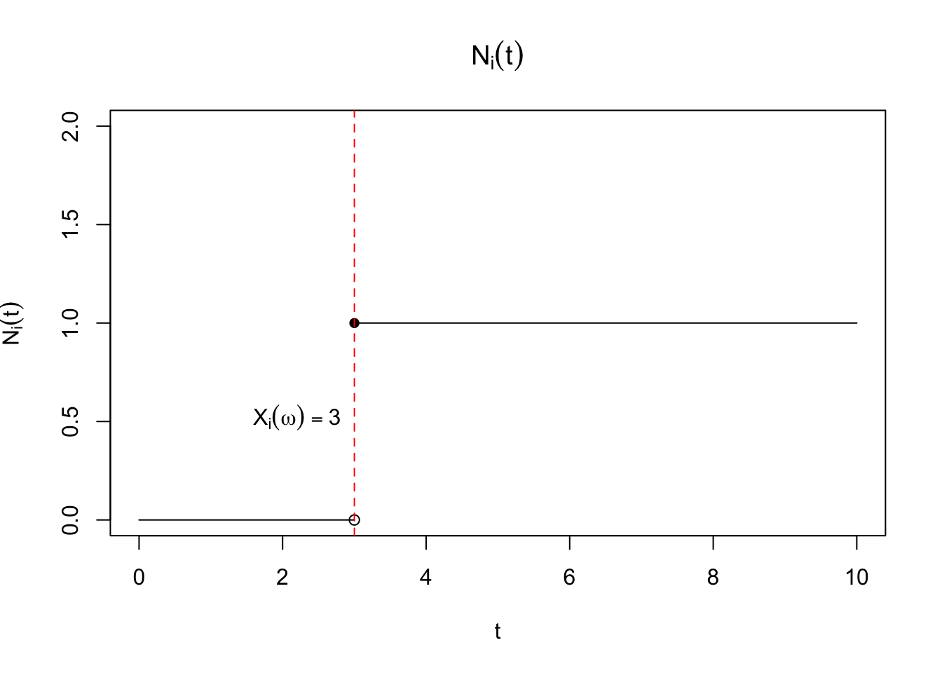
We’ve defined \(\delta_i\) as the indicator that the \(i^\mathrm{th}\) participant has experienced a failure over the course of the study. This is defined as \(\delta_i = \mathbbm{1}\left(X_i \leq C_i\right)\) where \(C_i\) is the time of censoring. We can imagine defining this variable for every time point \(t\) after the \(i^\mathrm{th}\) participant enters the study. Let \(N_i(t) = \mathbbm{1}\left(X_i \leq t, X_i \leq C_i\right)\). This equals \(\delta_i\) when \(t\) equals the study end point. On the event that \(X_i \leq C_i\), \(N_i(t)\) is a step-function of time, equalling \(0\) for all \(t \geq X_i\), and then jumping to \(1\) at \(t + \epsilon\) for all \(\epsilon > 0\). A plot of this function is shown in Figure 1. This variable can be seen to be a function of \(t\), and is technically called a stochastic process. One way to think about this is that \(N_i(t)\) is a random function of time. To see this note that for every draw of \(X_i\), \(N_i(t)\) is a different step function, jumping up to \(1\) at \(X_i\).

Figure 1: Example plot of \(N_i(t)=\mathbbm{1}\left(3 \leq t\right)\)

Of course, a natural quantity that arises from our definition is \[\Exp{N_i(t)} = \Exp{\mathbbm{1}\left(X_i \leq t,X_i \leq C_i\right)} = P(X_i \leq t, X_i \leq C_i).\] Let \(S_{C_i}(x)\) be the survival function of \(C_i\), or \(P(C_i > x)\) evaluated at \(x\), and let \(S_{X_i}(x)\) be the survival function of \(X_i\). Writing down the expression for the expectation of \(N_i(t)\) in terms of the hazard ratio for \(X_i\), \(\lambda_i(x)\), will show that the martingale residuals have mean zero: We’ll assume for ease of exposition that \(X_i \perp\!\!\!\perp C_i\). Remember that \(\lambda_i(x) = f_{X_i}(x)/S_{X_i}(x-)\), and that we’ve defined \(T_i = \min(X_i, C_i)\). Let the density function for \(T_i\) be \(f_{T_i}(y)\). \[\begin{align*} \Exp{N_i(t)} & = P(X_i \leq t, X_i \leq C_i) \\ & = \int_{0}^t S_{C_i}(x-) f_{X_i}(x) dx \\ & = \int_{0}^t S_{C_i}(x-) f_{X_i}(x) \frac{S_{X_i}(x-)}{S_{X_i}(x-)} dx \\ & = \int_{0}^t S_{C_i}(x-) S_{X_i}(x-)\frac{f_{X_i}(x)}{S_{X_i}(x-)} dx \\ & = \int_{0}^t P(C_i \geq x, X_i \geq x) \lambda_i(x) dx \\ & = \int_{0}^t \Exp{\mathbbm{1}\left(C_i \geq x, X_i \geq x\right)} \lambda_i(x) dx \\ & = \int_{0}^t \Exp{\mathbbm{1}\left(T_i \geq x\right)} \lambda_i(x) dx \quad (T_i = \min(X_i,C_i))\\ & = \int_{0}^t \mathbbm{1}\left(y \geq x\right) f_{T_i}(y) dy \lambda_i(x) dx \quad (T_i = \min(X_i,C_i))\\ & = \int_{0}^\infty \int_0^{\infty} \mathbbm{1}\left(t \geq x\right) \mathbbm{1}\left(y \geq x\right) f_{T_i}(y) dy\lambda_i(x) dx \\ & = \int_{0}^\infty \int_0^{\infty} \mathbbm{1}\left(t \geq x\right) \mathbbm{1}\left(y \geq x\right) \lambda_i(x) dx f_{T_i}(y) dy \text{ (Fubini)}\\ %& = \int_{0}^t \int_x^\infty f_{T_i}(y) dy \lambda_i(x) dx \\ %& = \int_{0}^\infty \int_0^{\min(t,y)} \lambda_i(x) dx f_{T_i}(y) dy \text{ (Fubini)}\\ %& = \int_{0}^\infty \int_0^{\infty} \ind{t \geq x} \ind{y \geq x} \lambda_i(x) dx f_{T_i}(y) dy\\ & = \int_{0}^\infty \int_0^{t} \mathbbm{1}\left(y \geq x\right) \lambda_i(x) dx f_{T_i}(y) dy\\ & = \Exp{\int_{0}^t \mathbbm{1}\left(T_i \geq x\right) \lambda_i(x) dx} \end{align*}\] It immediately follows that \[\Exp{N_i(t) - \int_{0}^t \lambda_i(x) \mathbbm{1}\left(T_i \geq x\right) dx} = 0.\]

3.2 Schoenfeld residuals

Instead, we can use the score equations above to generate residuals, called Schoenfeld residuals. Let \(z_{ik}\) be the \(k^\mathrm{th}\) component of the vector \(\mathbf{z}_i\), and let \[\hat{a}_{ik} = \frac{\sum_{j \in R(t_i)} z_{jk} \exp(\mathbf{z}_j^T \boldsymbol{\beta})}{ \sum_{j \in R(t_i)} \exp(\mathbf{z}_j^T \boldsymbol{\beta})}\] \[\begin{align} e^S_{ik} = \delta_i \left(z_{ik} - \hat{a}_{ik}\right) \end{align}\] These give some sense of how much the \(i^\mathrm{th}\) observation is contributing to the score equations for \(\beta_k\) at the MLE for \(\boldsymbol{\beta}\).

This residual highlights the conditional probability view of the Cox model. In this interpretation, the \(i^\mathrm{th}\) participant will be selected for failure at time \(t_i\) with probability: \[\begin{align} \frac{\exp(\mathbf{z}_i \boldsymbol{\beta})} {\sum_{j \in R(t_i)} \exp(\mathbf{z}_j^T \boldsymbol{\beta})} \end{align}\] This means, conditional on the set of observed values \(\mathbf{z}_j, j\in R(t_i)\), that \(\mathbf{z}_i\) is a random variable with a mean: \[\begin{align} \Exp{\mathbf{z}_i \mid R(t_i)} = \frac{\sum_{j \in R(t_i)} \mathbf{z}_j \exp(\mathbf{z}_j^T \boldsymbol{\beta})}{\sum_{j \in R(t_i)} \exp(\mathbf{z}_j^T \boldsymbol{\beta})} \end{align}\] and variance: \[\begin{align} \Var{\mathbf{z}_i \mid R(t_i)} = \frac{\sum_{j \in R(t_i)} \mathbf{z}_j\mathbf{z}_j^T \exp(\mathbf{z}_j^T \boldsymbol{\beta})}{\sum_{j \in R(t_i)} \exp(\mathbf{z}_j^T \boldsymbol{\beta})} - \Exp{\mathbf{z}_i \mid R(t_i)}^2 \end{align}\]

3.3 Testing proportional hazards

This view also can be used to show that these residuals can be used to determine whether the proportional hazards assumption is valid. For the rest of this section, for exposition purposes, let’s assume we have one covariate, \(z_i\). Suppose we are worried that our data may be generated by a model with a hazard ratio defined as \[\lambda_i(t) = \lambda_0(t) \exp(\beta z_i + g(t) \theta z_i)\] for some function \(g(t)\). Let the null hypothesis be that \(g(t) = 0\), and the alternative be that \(g(t) \neq 0\). If we write the true (unobservable) Schoenfeld residuals for this model we get: \[\epsilon^S_{i} = z_i - \ExpA{z_i \mid R(t_i)}{H_0}\] where \[\ExpA{z_i \mid R(t_i)}{H_0} = \frac{\sum_{j \in R(t_i)} z_j \exp(z_j \beta)}{\sum_{j \in R(t_i)} \exp(z_j \beta)}\] which we can expand with \[\epsilon^S_{i} = z_i - \frac{\sum_{j \in R(t_i)} z_j \exp(\beta z_j + g(t) \theta z_j)}{\sum_{j \in R(t_i)} \exp(\beta z_j + g(t) \theta z_j)} + \frac{\sum_{j \in R(t_i)} z_j \exp(\beta z_j + g(t) \theta z_j)}{\sum_{j \in R(t_i)} \exp(\beta z_j + g(t) \theta z_j)} - \ExpA{z_i \mid R(t_i)}{H_0}\]

Under this formulation \[\Exp{z_i - \frac{\sum_{j \in R(t_i)} z_j \exp(\beta z_j + g(t) \theta z_j)}{\sum_{j \in R(t_i)} \exp(\beta z_j + g(t) \theta z_j)} \mid R(t_i)} = 0\] by definition of the conditional expectation of \(z_i\). Let’s do a one-term Taylor expansion of the true conditional mean under the alternative model about \(g(t) = 0\): \[\begin{align*} \frac{\sum_{j \in R(t_i)} z_j \exp(\beta z_j + g(t) \theta z_j)}{\sum_{j \in R(t_i)} \exp(\beta z_j + g(t) \theta z_j)} & \approx \frac{\sum_{j \in R(t_i)} z_j \exp(\beta z_j)}{\sum_{j \in R(t_i)} \exp(\beta z_j)} + \frac{\partial}{\partial g(t)}\frac{\sum_{j \in R(t_i)} z_j \exp(\beta z_j + g(t) \theta z_j)}{\sum_{j \in R(t_i)} \exp(\beta z_j + g(t) \theta z_j)}\Bigg|_{g(t)=0}g(t) \\ & = \frac{\sum_{j \in R(t_i)} z_j \exp(\beta z_j)}{\sum_{j \in R(t_i)} \exp(\beta z_j)}\\ &\quad + g(t)\frac{\sum_{j \in R(t_i)} \theta z_j^2 \exp(\beta z_j + g(t) \theta z_j)}{\sum_{j \in R(t_i)} \exp(\beta z_j + g(t) \theta z_j)}\\ &\quad - g(t) \theta \frac{(\sum_{j \in R(t_i)} z_j \exp(\beta z_j + g(t) \theta z_j))^2}{(\sum_{j \in R(t_i)} \exp(\beta z_j + g(t) \theta z_j))^2}\Bigg|_{g(t) = 0} \\ & = \ExpA{z_i \mid R(t_i)}{H_0} + \VarA{z_i \mid R(t_i)}{H_0} \theta g(t) \end{align*}\] Plugging this in above gives: \[\epsilon^S_{i} \approx z_i - \frac{\sum_{j \in R(t_i)} z_j \exp(\beta z_j + g(t) \theta z_j)}{\sum_{j \in R(t_i)} \exp(\beta z_j + g(t) \theta z_j)} + \VarA{z_i \mid R(t_i)}{H_0} \theta g(t)\] Taking conditional expecations gives: \[\Exp{\epsilon^S_{i} \mid R(t_i)} \approx \VarA{z_i \mid R(t_i)}{H_0} \theta g(t)\] Using the plug-in estimator \(e^S_i\) for \(\Exp{\epsilon^S_{i} \mid R(t_i)}\) gives that \[e^S_i \approx \VarA{z_i \mid R(t_i)}{H_0} \theta g(t)\] under the alternative. Thus, plotting \(e^S_i\) against \(t\) gives a sense for whether there is evidence against the proportional hazards assumption.

Letting \(e^S_i = z_i - \ExpA{z_i \mid R(t_i)}{H_0}\) gives

3.4 Influence function for Cox PH model

Of course, we have a tool that will give another approximation of how much an individual observation contributes to the score equations, the influence function we derived in lecture 11. To make this more precise, we’ll need to define the weighted score equations: \[\begin{align} \nabla_{\beta} p\ell(\boldsymbol{\beta}, \mathbf{w}) = \sum_{i=1}^n w_i \delta_i \left(\mathbf{z}_i - \frac{\sum_{j \in R(t_i)} \mathbf{z}_j w_j \exp(\mathbf{z}_j^T \boldsymbol{\beta})}{ \sum_{j \in R(t_i)} w_j \exp(\mathbf{z}_j^T \boldsymbol{\beta})}\right) \end{align}\] The key thing to note is that the weight vector shows up in two places, because omitting an observation omits the observation from the risk set, against which other observations are measured. We can see this by rewriting the score equations for an observation indexed by \(k\). \[\begin{align} \nabla_{\beta} p\ell(\boldsymbol{\beta}, \mathbf{w}) = w_k \delta_k \left(\mathbf{z}_k - \frac{\sum_{j \in R(t_k)} \mathbf{z}_j w_j \exp(\mathbf{z}_j^T \boldsymbol{\beta})}{ \sum_{j \in R(t_k)} w_j \exp(\mathbf{z}_j^T \boldsymbol{\beta})}\right)+ \sum_{i\neq k}^n w_i \delta_i \left(\mathbf{z}_i - \frac{\sum_{j \in R(t_i)} \mathbf{z}_j w_j \exp(\mathbf{z}_j^T \boldsymbol{\beta})}{ \sum_{j \in R(t_i)} w_j \exp(\mathbf{z}_j^T \boldsymbol{\beta})}\right) \end{align} \tag{4}\] Then we take the gradient of Equation 4 with respect to \(w_k\). Note that \(w_k\) will show up for all risk sets prior to and including \(t_k\). Then we can write the gradient as: \[\begin{align*} \frac{\partial}{\partial w_k} \nabla_{\beta} p\ell(\boldsymbol{\beta}, \mathbf{w}) & = \delta_k \left(\mathbf{z}_k - \frac{\sum_{j \in R(t_k)} \mathbf{z}_j w_j \exp(\mathbf{z}_j^T \boldsymbol{\beta})}{ \sum_{j \in R(t_k)} w_j \exp(\mathbf{z}_j^T \boldsymbol{\beta})}\right)- w_k \delta_k \frac{\partial}{\partial w_k} \left(\frac{\sum_{j \in R(t_k)} \mathbf{z}_j w_j \exp(\mathbf{z}_j^T \boldsymbol{\beta})}{ \sum_{j \in R(t_k)} w_j \exp(\mathbf{z}_j^T \boldsymbol{\beta})}\right)\\ & - \quad \sum_{i \mid t_i < t_k} w_i \delta_i \frac{\partial}{\partial w_k} \left(\frac{\sum_{j \in R(t_i)} \mathbf{z}_j w_j \exp(\mathbf{z}_j^T \boldsymbol{\beta})}{ \sum_{j \in R(t_i)} w_j \exp(\mathbf{z}_j^T \boldsymbol{\beta})}\right)\\ & = \delta_k \left(\mathbf{z}_k - \frac{\sum_{j \in R(t_k)} \mathbf{z}_j w_j \exp(\mathbf{z}_j^T \boldsymbol{\beta})}{ \sum_{j \in R(t_k)} w_j \exp(\mathbf{z}_j^T \boldsymbol{\beta})}\right)- \sum_{i \mid t_i \leq t_k} w_i \delta_i \frac{\partial}{\partial w_k} \left(\frac{\sum_{j \in R(t_i)} \mathbf{z}_j w_j \exp(\mathbf{z}_j^T \boldsymbol{\beta})}{ \sum_{j \in R(t_i)} w_j \exp(\mathbf{z}_j^T \boldsymbol{\beta})}\right) \end{align*}\] The gradient of the second term is \[\begin{align} \frac{\partial}{\partial w_k} \left(\frac{\sum_{j \in R(t_i)} \mathbf{z}_j w_j \exp(\mathbf{z}_j^T \boldsymbol{\beta})}{ \sum_{j \in R(t_i)} w_j \exp(\mathbf{z}_j^T \boldsymbol{\beta})}\right)& = \frac{\mathbf{z}_k \exp(\mathbf{z}_k^T \boldsymbol{\beta})}{\sum_{j \in R(t_i)} w_j \exp(\mathbf{z}_j^T \boldsymbol{\beta})} \\ & - \exp(\mathbf{z}_k^T \boldsymbol{\beta})\frac{\sum_{j \in R(t_i)} \mathbf{z}_j w_j \exp(\mathbf{z}_j^T \boldsymbol{\beta})}{(\sum_{j \in R(t_i)} w_j \exp(\mathbf{z}_j^T \boldsymbol{\beta}))^2} \end{align}\] Putting this all back together gives us \[\begin{align*} \frac{\partial}{\partial w_k} \nabla_{\beta} p\ell(\boldsymbol{\beta}, \mathbf{w}) & = \delta_k \left(\mathbf{z}_k - \frac{\sum_{j \in R(t_k)} \mathbf{z}_j w_j \exp(\mathbf{z}_j^T \boldsymbol{\beta})}{ \sum_{j \in R(t_k)} w_j \exp(\mathbf{z}_j^T \boldsymbol{\beta})}\right)\\ & - \sum_{i \mid t_i \leq t_k} w_i \delta_i \frac{\exp(\mathbf{z}_k^T \boldsymbol{\beta})}{\sum_{j \in R(t_i)} w_j \exp(\mathbf{z}_j^T \boldsymbol{\beta})} \left(\mathbf{z}_k - \frac{\sum_{j \in R(t_i)} \mathbf{z}_j w_j \exp(\mathbf{z}_j^T \boldsymbol{\beta})}{\sum_{j \in R(t_i)} w_j \exp(\mathbf{z}_j^T \boldsymbol{\beta})} \right) \end{align*}\] Evaluating this term at \(w_i = 1 \forall i\) gives us \[\begin{align*} \frac{\partial}{\partial w_k} \nabla_{\beta} p\ell(\boldsymbol{\beta}, \mathbf{w})\Bigg|_{\mathbf{w}=1} & = \delta_k \left(\mathbf{z}_k - \frac{\sum_{j \in R(t_k)} \mathbf{z}_j \exp(\mathbf{z}_j^T \boldsymbol{\beta})}{ \sum_{j \in R(t_k)} \exp(\mathbf{z}_j^T \boldsymbol{\beta})}\right)\\ & - \sum_{i \mid t_i \leq t_k} \delta_i\frac{\exp(\mathbf{z}_k^T \boldsymbol{\beta})}{\sum_{j \in R(t_i)} \exp(\mathbf{z}_j^T \boldsymbol{\beta})} \left(\mathbf{z}_k - \frac{\sum_{j \in R(t_i)} \mathbf{z}_j \exp(\mathbf{z}_j^T \boldsymbol{\beta})}{\sum_{j \in R(t_i)} \exp(\mathbf{z}_j^T \boldsymbol{\beta})} \right) \end{align*}\] If we look at this for the \(m^\mathrm{th}\) element of \(\boldsymbol{\beta}\), we can rewrite it in terms of the Schoenfeld residuals and the terms \(\hat{a}_{im}\): \[\begin{align*} \left(\frac{\partial}{\partial w_k} \nabla_{\beta} p\ell(\boldsymbol{\beta}, \mathbf{w})\Bigg|_{\mathbf{w}=1}\right)_m & = e^S_{im} - \sum_{i \mid t_i \leq t_k} \delta_i\frac{\exp(\mathbf{z}_k^T \boldsymbol{\beta})}{\sum_{j \in R(t_i)} \exp(\mathbf{z}_j^T \boldsymbol{\beta})} \left(z_{km} - \hat{a}_{im} \right) \end{align*}\] This shows that the impact of leaving out one observation on the score equation is a) the direct effect of the observed failure for the \(k^\mathrm{th}\) unit had on the likelihood and b) the indirect effect of being excluded from the risk set; this impact occurs even if the \(k^\mathrm{th}\) patient is not observed to fail. The second term also increases in magnitude as the time at risk increases, so for patients at risk for a long time, this term typically outweighs the first term.