Lecture 2
1 Hazard function
Another way to characterize the random variable \(X_i\) is the hazard function, which is typically denoted as \(\lambda(t)\) or \(h(t)\) and is defined as \[\begin{align*} \lambda_{X_i}(t) & = \lim_{\Delta t \searrow 0}\frac{1}{\Delta t}\Prob{t \leq X_i < t + \Delta t \mid X_i \geq t}{\theta} \\ & = \lim_{\Delta t \searrow 0}\frac{1}{\Delta t}\frac{\Prob{t \leq X_i < t + \Delta t}{\theta}}{\Prob{X_i \geq t }{\theta}} \end{align*}\] First, note that we can define \(\Prob{X_i \geq t}{\theta}\) in terms of the survival function as: \[ \Prob{X_i \geq t}{\theta} = \lim_{s\nearrow t} S_{X_i}(s ;\, \theta). \] Using the notation introduced in the last lecture, we can write this as \[ \Prob{X_i \geq t}{\theta} = S_{X_i}(t- ;\, \theta). \] Of course, when \(X_i\) is absolutely continuous,\(S_{X_i}(t- ;\, \theta) = S_{X_i}(t ;\, \theta)\), but when \(X_i\) is discrete, or mixed discrete and continuous, as noted above, it is not true in general that the survival function is left-continuous.
A few things to note about \(\lambda_{X_i}(t ;\, \theta)\): when \(X_i\) is an absolutely continuous random variable, which occurs when we’re considering survival in continuous time, we can write this in terms of the probability density function \(f_{X_i}(t ;\, \theta)\) and the cumulative distribution function \(F_{X_i}(t ;\, \theta)\): \[\begin{align*} \lambda_{X_i}(t) & = \lim_{\Delta t \searrow 0}\frac{1}{\Delta t}\frac{\Prob{t \leq X_i < t + \Delta t}{\theta}}{\Prob{X_i \geq t}{\theta}} \\ & = \lim_{\Delta t \searrow 0}\frac{F_{X_i}(t + \Delta t;\, \theta) - F_{X_i}(t;\, \theta)}{\Delta t} \times \frac{1}{1 - F_{X_i}(t;\, \theta)} \\ & = \frac{f_{X_i}(t;\, \theta)}{1 - F_{X_i}(t;\, \theta)}. \end{align*}\] Let’s examine how the survival function and the hazard function fit together. \[ \lambda_{X_i}(t) = \frac{f_{X_i}(t ;\, \theta)}{S_{X_i}(t- ;\, \theta)}. \] Note that we can write the hazard function in terms of the survival function instead of the density, when \(X_i\) is absolutely continuous: \[\begin{align*} \lambda_{X_i}(t) & = \lim_{\Delta t \searrow 0}\frac{1}{\Delta t}\frac{\Prob{t \leq X_i < t + \Delta t}{\theta}}{\Prob{X_i \geq t}{\theta}} \\ & = \frac{1}{S_{X_i}(t ;\, \theta)} \times \lim_{\Delta t \searrow 0}\frac{S_{X_i}(t ;\, \theta)-S_{X_i}(t + \Delta t ;\, \theta) }{\Delta t} \\ & = \frac{1}{S_{X_i}(t ;\, \theta)} \times -\frac{d}{dt} S_{X_i}(t ;\, \theta). \end{align*}\] This implies that \[ \lambda_{X_i}(t) = -\frac{d}{dt} \log S_{X_i}(t ;\, \theta). \] If we integrate both sides, we get another important identity in survival analysis: \[\begin{align} \int_{0}^u \frac{d}{dt} \log S_{X_i}(t ;\, \theta) dt & = -\int_{0}^u\lambda_{X_i}(t) dt \\ \log S_{X_i}(u ;\, \theta) - \log S_{X_i}(0 ;\, \theta) & = -\int_{0}^u\lambda_{X_i}(t) dt \quad \text{note}\,\,\, S_{X_i}(0 ;\, \theta) = 1\\ S_{X_i}(u ;\, \theta) & = \exp \lp -\int_{0}^u\lambda_{X_i}(t) dt\rp \label{eq:exp-hazard} \end{align}\]
1.1 Properties of the hazard function
The relationship \(S_{X_i}(u;\,\theta) = \exp \lp -\int_{0}^u\lambda_{X_i}(t) dt\rp\) and the properties of the survival function reveal the following facts about the hazard function and highlight its differences with a probability density.
\(\lim_{t\to\infty} S_{X_i}(t;\,\theta) = 0\) implies that \(\lim_{t\to\infty} \int_0^t \lambda_X(u) du = \infty\)
Given that \(S_{X_i}(t;\,\theta)\) is a nonincreasing function, \(\lambda_X(t) \geq 0\) for all \(t\).
So unlike a probability density function, \(\lambda_X(t)\) isn’t integrable over the support of the random variable.
2 Density function for survival time
Given that we have \(S_{X_i}(t;\,\theta)\) and \(\lambda(t) = \frac{f_{X_i}(t;\,\theta)}{S_{X_i}(t-;\,\theta)}\), we can recover the density, \(f_{X_i}(t;\,\theta)\) easily: \[ f_{X_i}(t;\,\theta) = \lambda_{X_i}(t) S_{X_i}(t-;\,\theta) \]
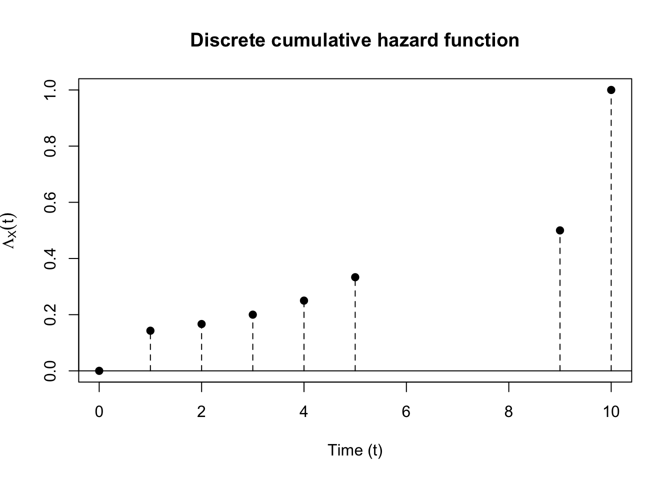
3 Cumulative hazard function
One final important quantity that describes a survival distribution is that of cumulative hazard, which we’ll denote as \(\Lambda_{X_i}(t)\), though it is also denoted as \(H(t)\) in . This is defined as you might expect: \[ \Lambda_{X_i}(t) = \int_{0}^t \lambda_{X_i}(u) du. \] It has the important property that for any absolutely continuous failure time \(X_i\) with a given cumulative hazard function, the random variable \(Y_i = \Lambda_{X_i}(X_i)\) is exponentially distributed with rate \(1\). The derivation is straightforward. Remember that \(P(X_i > t) = \exp\lp-\Lambda_{X_i}(t)\rp\) \[\begin{align*} P(\Lambda_{X_i}(X_i) > t) & = P(X_i > \Lambda_{X_i}^{-1}(t)) \\ & = \exp\lp-\Lambda_{X_i}(\Lambda_{X_i}^{-1}(t))\rp \\ & = \exp\lp-t\rp \end{align*}\]
4 Discrete survival time
We’ve been working with continuous survival times until now. If \(X_i\) is a discrete random variable with support on \(\{t_1, t_2, \dots\}\), we lose some of the tidyness of the previous derivations. We can define the distribution of \(X_i\) in terms of the survival function, \(P_{\theta}(X_i > t)\). First let \(p_j = P_{\theta}(X_i = t_j)\), so \[ S_{X_i}(t;\,\theta) = P_{\theta}(X_i > t) = \sum_{j \mid t_j > t} p_j \] We can also define the hazard function for a discrete random variable: \[ \lambda_{X_i}(t_j) = \frac{p_j}{S_{X_i}(t_{j-1};\,\theta)} = \frac{p_j}{p_j + p_{j+1} + \dots} \] Note that \(p_j = S_{X_i}(t_{j-1};\,\theta) - S_{X_i}(t_{j};\,\theta)\), then \[ \lambda_{X_i}(t_j) = 1 - \frac{S_{X_i}(t_j;\,\theta)}{S_{X_i}(t_{j-1};\,\theta)}. \] If we let \(t_0 = 0\) then \(S_{X_i}(t_0;\,\theta) = 1\). This allows us to write the survival function in a sort of telescoping product: \[\begin{align*} P_{\theta}(X_i > t_j) & = P_{\theta}(X_i > t_0) \frac{P_{\theta}(X_i > t_1)}{P_{\theta}(X_i > t_0)} \frac{P_{\theta}(X_i > t_2)}{P_{\theta}(X_i > t_1)} \dots \frac{P_{\theta}(X_i > t_j)}{P_{\theta}(X_i > t_{j-1})} \\ & = 1 \frac{S_{X_i}(t_1;\,\theta)}{S_{X_i}(t_0;\,\theta)}\frac{S_{X_i}(t_2;\,\theta)}{S_{X_i}(t_1;\,\theta)} \dots \frac{S_{X_i}(t_j;\,\theta)}{S_{X_i}(t_{j-1};\,\theta)} \end{align*}\] This yields another way to write \(S_{X_i}(t;\,\theta)\):
\[ \begin{align} S_{X_i}(t;\,\theta) = \prod_{j \mid t_j \leq t} (1 - \lambda_{X_i}(t_j)). \end{align} \tag{1}\]
It turns out that we can write the survival function for continuous random variables in the same way.
4.1 Connection between discrete and continuous survival functions
Recall the definition of the hazard function:
\[ \lambda_{X_i}(t) = \lim_{\Delta t \searrow 0}\frac{1}{\Delta t}\Prob{t \leq X < t + \Delta t \mid X \geq t}{\theta} \] Note that \(\lambda_{X_i}(t) \,\Delta t\) is approximately \(\Prob{t \leq X < t + \Delta t \mid X \geq t}{\theta}\). Let \(\mathcal{T}\) be a partition of \((0,\infty)\) with partition size \(\Delta t\), \(t_0 = 0\), \(t_j = t_{j-1} + \Delta t\): \[ \mathcal{T} = \bigcup_{j=0}^\infty [t_j, t_j + \Delta t). \] Then we can use Equation 1 to represent the survival function: \[\begin{align} S_{X_i}(t;\,\theta) = \prod_{j \mid t_j + \Delta t \leq t} (1 - \lambda_{X_i}(t_j)\Delta t). \end{align}\] We can show that as the partition of the time domain gets finer and finer, we will recover \(S_{X_i}(t;\,\theta) = \exp(-\int_0^t\lambda_{X_i}(u)du)\) \[\begin{align} S_{X_i}(t;\,\theta) & = \prod_{j \in \mathcal{T} \mid t_j + \Delta t \leq t} (1 - \lambda_{X_i}(t_j)\Delta t) \\ \log S_{X_i}(t;\,\theta)& = \sum_{j \in \mathcal{T} \mid t_j + \Delta t \leq t} \log(1 - \lambda_{X_i}(t_j)\Delta t) \end{align}\] We use the Taylor expansion of \(\log(1 - \lambda_{X_i}(t_j) \Delta t)\) for small \(\lambda_{X_i}(t_j) \Delta t\), assuming that \(\lambda_{X_i}(t)\) is sufficiently well-behaved for all \(t\). \[ \log(1 - \lambda_{X_i}(t_j) \Delta t) \approxeq -\lambda_{X_i}(t_j) \Delta t. \] Then \[\begin{align} \log S_{X_i}(t;\,\theta)& \approxeq \sum_{j \in \mathcal{T} \mid t_j + \Delta t \leq t} -\lambda_{X_i}(t_j)\Delta t \end{align}\] As \[ \lim_{\Delta t \searrow 0} \sum_{j \in \mathcal{T} \mid t_j + \Delta t \leq t} -\lambda_{X_i}(t_j)\Delta t = -\int_0^t \lambda_{X_i}(u) du. \] So, \(S_{X_i}(t;\,\theta) = \exp(-\int_0^t\lambda_{X_i}(u)du)\), or \[\begin{align}\label{eq:suvival-exp-cumulative-hazard} S_{X_i}(t;\,\theta) = \exp(-\lambda_{X_i}(t)) \end{align}\]
5 Mean residual lifetime
We also might be interested in the mean residual lifetime (mrl for short), or the expected lifetime given survival up to a certain point: \[ \Exp{X_i - x \mid X_i > x}. \] We can compute this for an absolutely continuous random variable by using the survival function: \[\begin{align*} \frac{\int_{x}^\infty (u - x) f_{X_i}(u ;\, \eta) du}{S_{X_i}(x;\, \eta)} = \frac{\int_x^\infty S_{X_i}(u;\, \eta) du }{S_{X_i}(x;\, \eta)} \end{align*}\] To derive the mrl in terms of the survival function, note that we can use Fubini again on the numerator (Exercise 1), or we can use integration by parts: \[\begin{align*} \int_{x}^\infty (u - x) f_{X_i}(u) du & = -\int_{x}^\infty (u - x) \frac{d}{du} S_{X_i}(u) du \\ & = \left.-(u-x) S_{X_i}(u)\right\rvert_{u=x}^\infty + \int_x^\infty S_{X_i}(u) du \end{align*}\] and use the fact that \(\lim_{u\to\infty} S_{X_i}(u) = 0\). We also need the following: \[ \begin{align} \lim_{u\to\infty} u P(X_i > u) = 0. \end{align} \tag{2}\] This is a pretty weak condition, random variables with second moments satisfy this condition (Exercise 2), as do random variables with only first moments. It turns out that under this condition we’ll have a weak law of large numbers (see 7.1 in Resnick (2019)).
Suppose we assume that \(\Exp{X} \leq \infty\). Then we can write: \[ \Exp{X} = \Exp{X \ind{X \leq n}}+\Exp{X \ind{X > n}} \] Note that if we define \(X_n = X \ind{X \leq n}\) then \[ X_1(\omega) \leq X_2(\omega) \leq \dots \leq X_k(\omega) \leq \dots. \] By the Monotone Convergence Theorem (MCT), \(\Exp{X_n} \to \Exp{X}\). Then \[\begin{align*} \Exp{X} & = \Exp{X_n}+\Exp{X \ind{X > n}} \\ & \geq \Exp{X_n}+\Exp{n \ind{X > n}} \\ & = \Exp{X_n}+n P(X > n) \end{align*}\] This leads to the system of inequqalities: \[\begin{align*} \Exp{X} - \Exp{X_n} \geq n P(X > n) \geq 0. \end{align*}\]
By the MCT \(\Exp{X} - \Exp{X_n} \to 0\) so \[ \lim_{n\to\infty} n P(X_i > n) = 0. \] However, there are random variables for which \(\Exp{X_i}\) does not exist, but do satisfy Equation 2 (see the end of 7.1 in Resnick (2019)).
6 Parametric examples
The first example we’ll run through is for an exponentially distributed survival time: \[X_i \overset{\mathrm{iid}}{\sim} \mathrm{Exp}(\lambda).\] The survival function is \(S_{X}(t) = e^{-\lambda t}\). We can read off from this that \(\Lambda(t) = \lambda t\). What’s the hazard function? Let’s plot the hazard function. What does this imply about the exponential distribution (memorylessness)? The mean lifetime is \(\frac{1}{\lambda}\). The mean residual lifetime is: \[\begin{align*} \frac{\int_{t}^\infty e^{-\lambda u} du}{e^{-\lambda t}} & = \frac{1}{\lambda}\frac{e^{-\lambda t}}{e^{-\lambda t}} \\ & = \frac{1}{\lambda}. \end{align*}\] This is a consequence of the memoryless property of the exponential distribution.
Another parametric distribution for survival times is the Weibull. \[X_i \overset{\mathrm{iid}}{\sim} \mathrm{Weibull}(\gamma, \alpha).\] The survival function: \[ S_X(t) = \exp(-\gamma t ^ \alpha). \] Again, we have that \(\Lambda(t) = \gamma t ^ \alpha\), so we can take the derivative with respect to \(t\) to get the hazard: \[ \lambda(t) = \gamma \alpha t^{\alpha - 1}. \] This is more flexible than the exponential distribution, though note that for \(\alpha = 1\), \(X_i \sim \text{Exponential}(\gamma)\), so the Weibull family contains the exponential family as a special case. The \(\alpha\) parameter allows for the hazard rate to have more flexibility than the exponential. If \(\alpha > 1\), the hazard rate is increasing in \(t\). This corresponds to an aging process, whereby the longer something has survived, the higher the rate of failure. If \(\alpha < 1\), the hazard rate is decreasing in \(t\). This might correspond to something like the hazard for SIDS, which is quite high for children before 1 year old, but drops off rapidly after 1. Let’s compute the mean lifetime, \(\Exp{X} = \int_0^\infty S_X(t) dt\), using a \(v\)-sub, \(v = t^\alpha\), so \(v^{\frac{1}{\alpha}} = t \to \frac{1}{\alpha} v^{\frac{1}{\alpha} - 1} dv = dt\): \[\begin{align*} \int_0^\infty \exp(-\gamma t ^ \alpha)dt & = \frac{1}{\alpha} \int_0^\infty v^{\frac{1}{\alpha} - 1} \exp(-\gamma v)dv \\ & = \frac{1}{\alpha} \frac{1}{\gamma^{\frac{1}{\alpha}}} \Gamma(\frac{1}{\alpha}) \\ & = \frac{\Gamma(\frac{1}{\alpha} + 1)}{\gamma^{\frac{1}{\alpha}}} \end{align*}\] The mean residual lifetime is a bit more involved. Let \(v = \gamma u^\alpha\) so \(\lp\frac{v}{\gamma}\rp^{1/\alpha} = u \to \gamma^{-1/\alpha}\frac{1}{\alpha} v^{\frac{1}{\alpha} - 1} dv = du\): \[\begin{align*} \int_t^\infty \exp(-\gamma u ^ \alpha)du & = \gamma^{-1/\alpha}\frac{1}{\alpha} \int_{\gamma t^\alpha}^\infty v^{\frac{1}{\alpha} - 1} \exp(-v)dv \\ & = \gamma^{-1/\alpha}\frac{1}{\alpha} \Gamma(\frac{1}{\alpha}, \gamma t^\alpha), \end{align*}\] where \(\Gamma(\frac{1}{\alpha}, \gamma t^\alpha)\) is the upper incomplete Gamma function.
References
Resnick, Sidney. 2019. A Probability Path. Springer.