Lecture 3
1 Censoring and truncation
Now let’s delve into more detail about censoring, and how the likelihood can be built up from the hazard function and the survival function. define censoring as imprecise knowledge about an event time. If we observe a failure or an event exactly, the observation is not censored, but if we know only that an observation occurred within a range of values, we say the observation is censored. Let \(X_i\), as usual, be our failure time, which is not completely observed. Instead if:
\(X_i \in [C, \infty)\), the observation is right censored
\(X_i \in [0, U)\), the observation is left censored
\(X_i \in [C, U)\), the observation is interval censored
2 Right censoring
Right censoring occurs when a survival time is known to be larger than a given value. This is the most common censoring scenario in survival analysis.
Recall our definition in Lecture 1:
Let \(X_i\) be the time to failure, or time to event for individual \(i\).
Let \(C_i\) be the time to censoring. It may be helpful to think about \(C_i\) as the time to investigator measurement.
Let \(\delta_i = \ind{X_i \leq C_i}\).
Let \(T_i = \min(X_i, C_i)\). This implies that the event \(\{T_i \geq t\} \equiv \{C_i \geq t, X_i \geq t\}\).
Note that another way to write \(\min(X_i, C_i)\) is \(X_i \wedge C_i\). We’ll also see \(\max(X_i, C_i) \equiv X_i \vee C_i\).
Given our definitions above, when an observation is censored, or when a measurement is taken of the survival time before the event has happened, \(\delta_i = 0\) and \(T_i = C_i\).
2.1 Type I censoring
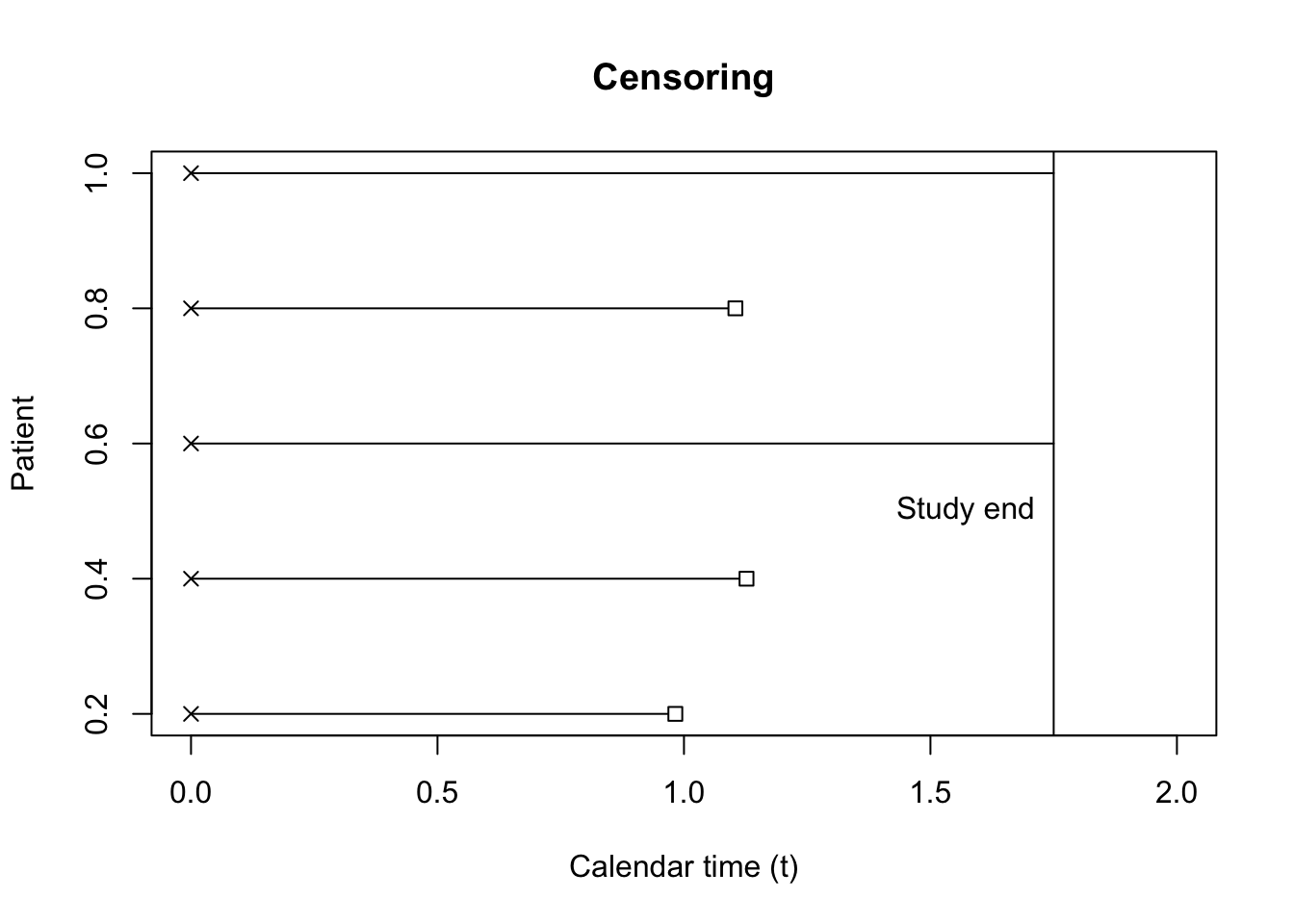
The simplest censoring scenario is one in which all individuals have the same, nonrandom censoring time. Imagine a study is designed to follow \(5\) startups that are spun out of a tech incubator to study how long it takes a company to land its first contract. This information will be used for designing investments \(2\) years from the study date, so the study has a length of \(1.75\) years. We can say that all observations will have to have occurred, or not, by \(1.75\) years.
Figure 1 shows a potential result of the study, where \(2\) out of the \(5\) companies have not landed a contract.
In this case, - For all individuals such that \(\delta_i = 0 \implies X_i > C\)
- \(\delta_i = 1 \implies T_i = X_i\).
2.2 Generalized type I censoring
A more general scenario, which is closer to most examples in clinical trials, is when each individual has a different study entry time and the investigator has a preset study end time. This is called generalized Type I censoring. These study entry times are typically assumed to be independent of the survival time. This is shown in Figure 2.
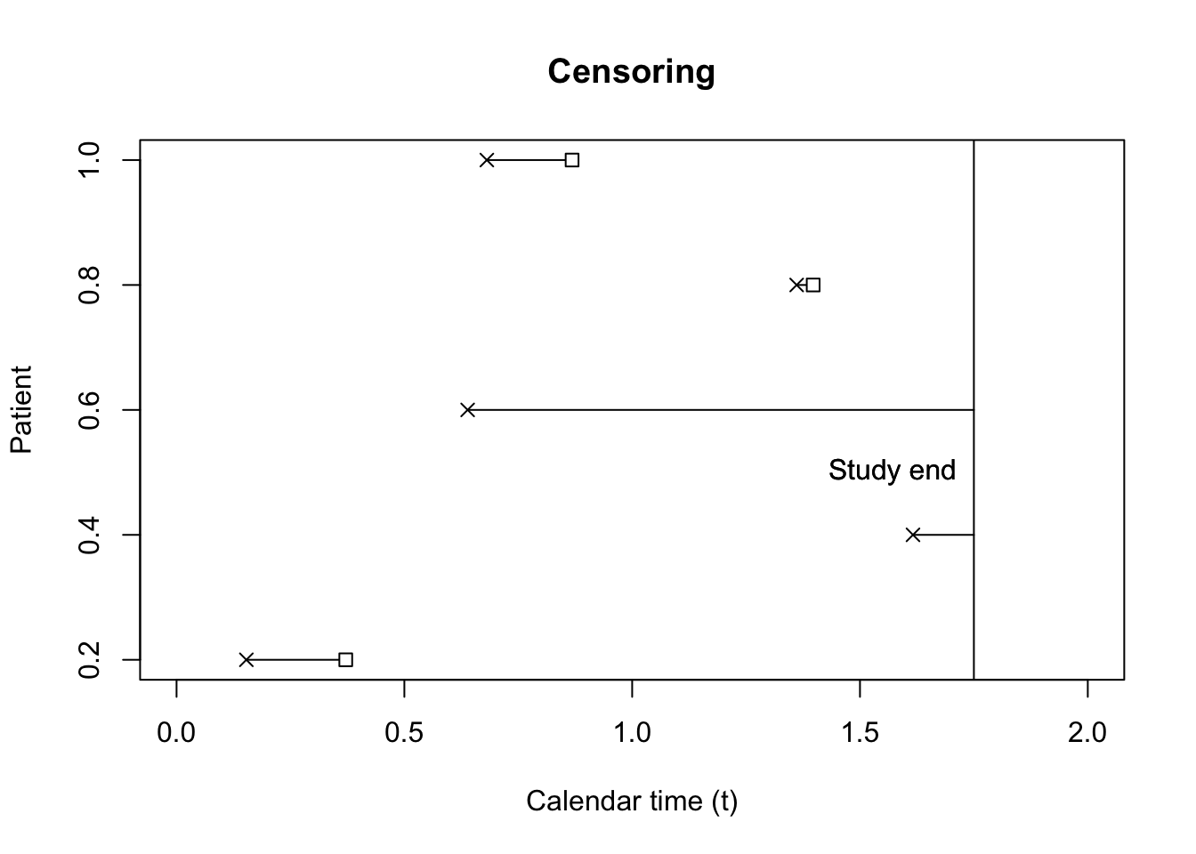
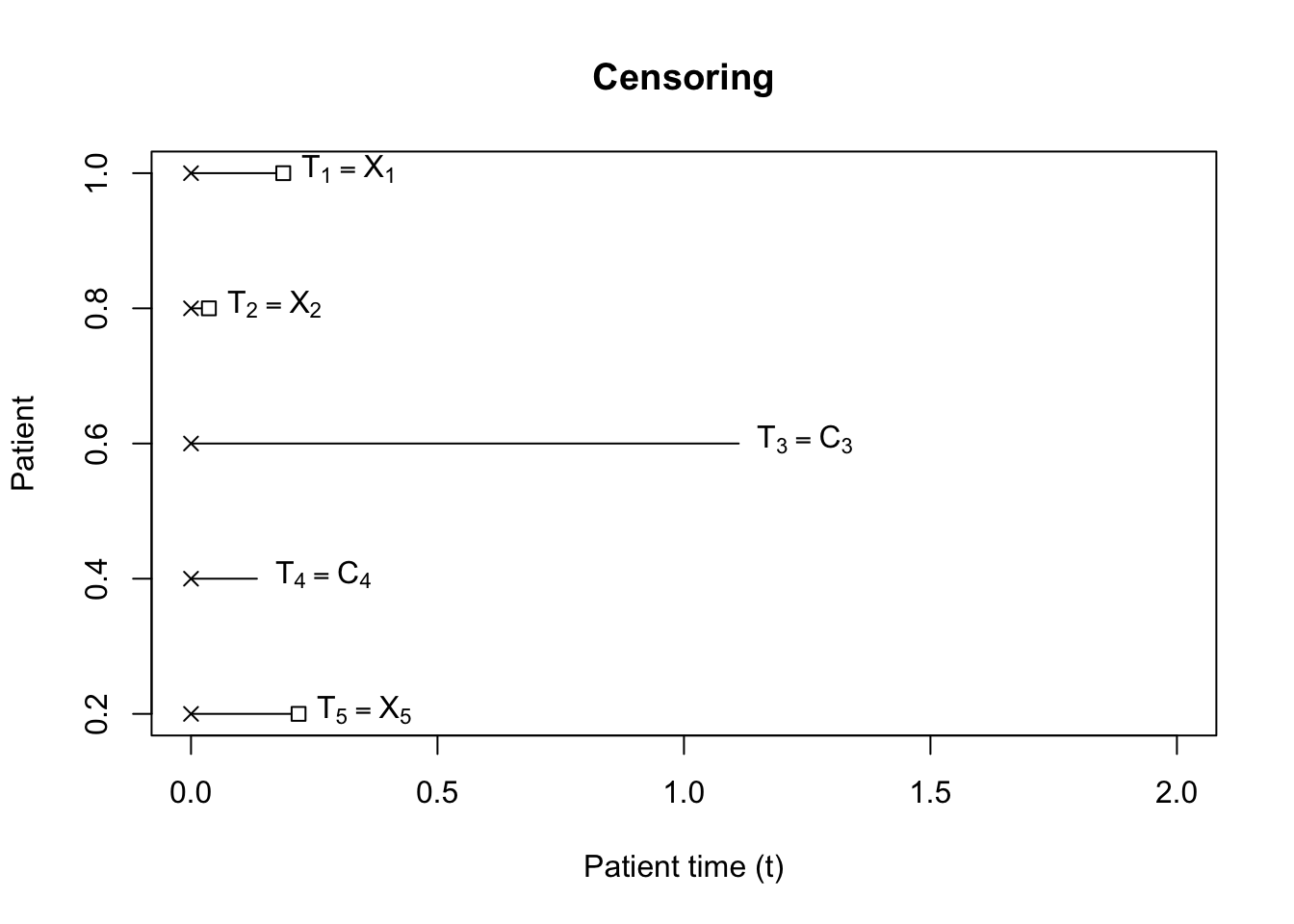
When study entry is independent from survival time, the analysis proceeds as shown in Figure 3.
For generalized type I censoring, - For all individuals such that \(\delta_i = 0 \implies X_i > C_i\)
- \(\delta_i = 1 \implies T_i = X_i\).
This is different from Type I censoring in that each individual has a different censoring time.
2.3 Type II censoring
Type II censoring occurs when all units have the same study entry time, but researchers design the study to end when \(r < n\) units fail out of \(n\) total units under observation.
For the first \(r\), lucky or unlucky participants, \(\delta_i = 1 \implies T_i = X_{(i)}\) or the \(i^\mathrm{th}\) order statistic.
For the remaining \(n - r\) individuals, \(\delta_i = 0 \implies X_i > X_{(r)}\).
2.4 Generalized Type II censoring
You may be wondering, what happens when units have differing start times but we want to end the trial after the \(r\)-th failure? It turns out that this was not a solved problem until Rühl, Beyersmann, and Friedrich (2023), which was quite surprising to me.
2.5 Independent censoring
A third type of censoring, helpfully called independent censoring, takes \(X_i \indy C_i\), and thus conclusions similar to those of generalized type I censoring can be drawn:
For all individuals such that \(\delta_i = 0 \implies X_i > C_i\)
\(\delta_i = 1 \implies T_i = X_i\).
3 Noninformative censoring
All of the previous censoring scenarios can be summarized as noninformative censoring. Let the parameters indexing the censoring distribution be \(\phi\), while the parameters indexing the failure time distribution are \(\eta\). Noninformative censoring is defined as the following equality: \[ \begin{aligned} \lambda_{X_i}(t) = \lim_{\Delta t \searrow 0} \frac{1}{\Delta t}\Prob{t \leq X_i < t + \Delta t \mid X_i \geq t, C_i \geq t}{\eta, \phi} \end{aligned} \tag{1}\] Note that this implies the following:
\[ \begin{aligned} \Prob{t \leq X_i < t + \Delta t \mid X_i \geq t}{\eta} = \Prob{t \leq X_i < t + \Delta t \mid X_i \geq t, C_i \geq t}{\eta, \phi}. \end{aligned} \tag{2}\] which is equivalent to writing
\[ \begin{aligned} \Prob{t \leq X_i < t + \Delta t \mid X_i \geq t}{\eta} = \Prob{t \leq T_i < t + \Delta t, \delta_i = 1 \mid T_i \geq t}{\eta, \phi}. \end{aligned} \] Another useful expression for the RHS is the following: \[ \begin{aligned} \Prob{t \leq X_i < t + \Delta t \mid X_i \geq t, C_i \geq t}{\eta, \phi} & = \frac{\Prob{t \leq X_i < t + \Delta t, C_i \geq t}{\eta, \phi}}{\Prob{X_i \geq t, C_i \geq t}{\eta, \phi}}\\ & = \frac{\Prob{X_i \geq t, C_i \geq t}{\eta, \phi} - \Prob{X_i \geq t + \Delta t, C_i \geq t}{\eta, \phi}}{\Prob{X_i \geq t, C_i \geq t}{\eta, \phi}} \end{aligned} \tag{3}\]
For independent censoring, Equation 2 holds, given that \(P_{\eta, \phi}(X_i > t, C_i > c) = P_{\eta}(X_i > t) P_{\phi}(C_i > c)\) and that \(\eta\) and \(\phi\) are variationally independent.
This means that the parameter space \(\Omega_{\eta,\phi}\) is the Cartesian product of the parameter space for \(\eta\) and \(\phi\).
Definition 1 (Variational independence) Let \(\eta \in \Omega_{\eta}\) and \(\phi \in \Omega_{\phi}\). The joint space is denoted as \(\Omega_{\eta, \phi}\). If \(\Omega_{\eta, \phi} = \Omega_\eta \times \Omega_\phi\), \(\eta\) and \(\phi\) are variationally independent. In other words, the range for \(\eta\) does not change given a value for \(\phi\).
Under independent censoring, the observable hazard for uncensored failure times is as follows: \[\begin{align} \frac{-\frac{\partial}{\partial u} P_{\eta, \phi}(X_i > u, C_i > t-) \mid_{u=t}}{P_{\eta,\phi}(X_i > t-, C_i > t-)} = \frac{-\frac{d}{du} S_{X_i}(u;\, \eta)}{S_{X_i}(t-;\, \eta)} \end{align}\]
Here’s an example that demonstrates the nonidentifiability of the joint distribution for censoring and failure time:
First, let’s define identifiability:
Definition 2
Example 1 (Dependent failure and censoring) Let \(P_{\theta,\alpha, \mu}(X_i > x, C_i > c) = \exp(-\alpha x - \mu c - \theta x c)\). We can find the marginal survival functions just by evaluating \(P_{\theta,\alpha, \mu}(X_i > x, C_i > 0)\) and vice-versa, which yields: \[\begin{align*} P_{\alpha}(X_i > x) & = \exp(- \alpha x) \\ P_{\mu}(C_i > c) & = \exp(- \mu c) \end{align*}\] Both of these distributions have constant hazards. However, the observable hazard is the following: \[\begin{align*} \frac{-\frac{\partial}{\partial u} P_{\theta,\alpha, \mu}(X_i > u, C_i > t-) \mid_{u=t}}{P_{\theta,\alpha, \mu}(X_i > t-, C_i > t-)} & = \alpha + \theta t \\ \frac{-\frac{\partial}{\partial u} P_{\theta,\alpha, \mu}(X_i > t-, C_i > u) \mid_{u=t}}{P_{\theta,\alpha, \mu}(X_i > t-, C_i > t-)} & = \mu + \theta t \\ \end{align*}\] This leads to an observable survival function: \[\begin{align*} S_{X_i}(x;\, \alpha, \theta) & = \exp(- \alpha x - \theta x^2/ 2 ) \\ S_{C_i}(c;\, \mu, \theta) & = \exp(- \mu c - \theta c^2 / 2) \end{align*}\] If we mistakenly assume that the failure time and the censoring time are independent we’ll get the following joint distribution: \[ S_{X_i}(x;\, \alpha, \theta) S_{C_i}(c;\, \mu, \theta) \neq \exp(-\alpha x - \mu c - \theta x c). \]
However, if we calculate the true observable survival function \(P_{\theta,\alpha, \mu}(X_i > x, C_i > X_i-)\) we get: \[\begin{align*} \int_x^\infty -\frac{\partial}{\partial u} P_{\theta,\alpha, \mu}(X_i > u, C_i > t-) \mid_{u=t} dt & = \int_x^\infty (\alpha + \theta t) \exp(-\alpha t - \mu t - \theta t^2) dt \end{align*}\] while the observable survival function implied the by the erroneously assumed independent distributons is: \[\begin{align*} \int_x^\infty -\frac{\partial}{\partial u} S_{X_i}(u;\, \alpha, \theta) \mid_{u=t} S_{C_i}(t-;\, \mu, \theta) dt & = \int_x^\infty (-\frac{d}{du}\exp(- \alpha u - \theta u^2 / 2 ))\mid_{u=t}\exp(- \mu t - \theta t^2/ 2 )dt \\ & = \int_x^\infty (\alpha + \theta t) \exp(-\alpha t - \mu t - \theta t^2) dt \end{align*}\]
Thus, two different joint densities lead to the same observable survival functions, so the joint distribution is nonidentifiable.
Here is an example showing that we may have dependent censoring and failure times, but still end up with noninformative censoring:
Example 2 (Dependent failure and censoring can be noninformative) Let \(Y_1, Y_2\) and \(Y_{12}\) be exponentially distributed with rates \(\alpha_1, \alpha_2, \alpha_{12}\), respectively. Let \(X = Y_1 \wedge Y_{12}\) and \(C = Y_2 \wedge Y_{12}\). The survival function \(P_{\alpha_1, \alpha_2, \alpha_{12}}(X > x, C > c) = P(Y_1 > x, Y_2 > c, Y_{12} > x \vee c) = e^{-\alpha_1 x -\alpha_2 c - \alpha_{12} x \vee c}\) Then marginally \(X\) is exponential with rate \(\alpha_1 + \alpha_{12}\), which is also equal to its hazard function. In order for noninformative censoring to hold, we need to check the definition Equation 1, or that \[\begin{align} \alpha_1 + \alpha_{12} = \lim_{\Delta t \searrow 0} \frac{1}{\Delta t} \Prob{t \leq X < t + \Delta t \mid X \geq t, C \geq t}{\alpha_1, \alpha_2, \alpha_{12}} \end{align}\] Representing \[ \begin{aligned} & \Prob{t \leq X < t + \Delta t \mid X \geq t, C \geq t}{\alpha_1, \alpha_2, \alpha_{12}}\\ & = \frac{\Prob{X_i \geq t, C_i \geq t}{\alpha_1, \alpha_2, \alpha_{12}} - \Prob{X_i \geq t + \Delta t, C_i \geq t}{\alpha_1, \alpha_2, \alpha_{12}}}{\Prob{X_i \geq t, C_i \geq t}{\alpha_1, \alpha_2, \alpha_{12}}} \end{aligned} \] and noting that \(t + \Delta t \vee t = t + \Delta t\) as \(\Delta t > 0\), \[\begin{align} \lim_{\Delta t \searrow 0} \frac{\Prob{X \geq t, C \geq t}{\alpha_1, \alpha_2, \alpha_{12}} - \Prob{X \geq t + \Delta t, C \geq t}{\alpha_1, \alpha_2, \alpha_{12}}}{\Delta t} = \lim_{\Delta t \searrow 0}\frac{e^{-\alpha_1 t -\alpha_2 t - \alpha_{12} t} - e^{-(\alpha_1 + \alpha_{12})(t + \Delta t) -\alpha_2 t}}{\Delta t} \end{align}\] which just equals \(e^{-\alpha t}(-\frac{d}{ds} e^{-(\alpha_1 + \alpha_{12})s} \mid_{s = t})\) or \((\alpha_1 + \alpha_{12})e^{-\alpha_1 t -\alpha_2 t - \alpha_{12} t}\). The denominator of the hazard rate is \(e^{-\alpha_1 t -\alpha_2 t - \alpha_{12} t}\).
Then \[\begin{align} \lim_{\Delta t \searrow 0} \frac{1}{\Delta t} \Prob{t \leq X < t + \Delta t \mid X \geq t, C \geq t}{\alpha_1, \alpha_2, \alpha_{12}} & = \frac{(\alpha_1 + \alpha_{12})e^{-\alpha_1 t -\alpha_2 t - \alpha_{12} t}}{e^{-\alpha_1 t -\alpha_2 t - \alpha_{12} t}} \\ & = \alpha_1 + \alpha_{12} \end{align}\] So in this case, while \(X\) and \(C\) are dependent, we still have noninformative censoring.
The benefit of noninformative censoring is that we can ignore the censoring random variables when constructing the likelihood for the survival random variables.
3.1 Reasons for informative censoring
A simple hypothetical situation with informative censoring would be one in which sick patients are lost to follow-up.
4 Truncation
While censoring can be seen as partial information about an observation, truncation deals with exact observations of selected units. The simplest example of truncation is when measurements are made using an instrument with a lower limit of detection. Imagine using a microscope to measure the diameter of cells on a plate that has a lower limit of detection of 5 microns. If interest lies in inferring the population mean diameter of the cells, one must take into account the fact that only cells with diameters of greater than 5 microns can be seen with the microscope.
Failure to take truncation into account can be a source of bias in inference. Let the lower bound of truncation be \(V\).
\[\begin{align*} \Exp{X_i} & = \Exp{X_i \mid X_i \geq V} P(X_i \geq V) + \Exp{X_i \mid X_i < V} P(X_i < V) \\ & = \Exp{X_i \mid X_i \geq V} + P(X_i < V) (\Exp{X_i \mid X_i < V} - \Exp{X_i \mid X_i \geq V}) \\ & \leq \Exp{X_i \mid X_i \geq V} \end{align*}\] The last line follows because \((\Exp{X_i \mid X_i < V} - \Exp{X_i \mid X_i \geq V}) \leq 0\). Using an estimator for \(\Exp{X_i \mid X_i \geq V}\) when the target of inference in \(\Exp{X_i}\) would result in positive bias. Of course, when the estimator instead estimates \(\Exp{X_i \mid X_i < V}\) the bias would be negative. Depending on the value of \(V\) and the distribution of \(X_i\), the bias can be severe.
For example, suppose a researcher is interested in learning about the impact of medication refills on the lifespans of patients. The researcher has access to a database in which they select patients who refilled medications at least once. The researcher subsequently selects a control group that is perfectly matched to the medication refill group, and upon analyzing the data, the analyst discovers that refilling prescription medication leads to longer lifespans. What is wrong with this analysis?
The observations in this example can be said to be left-truncated, because the researcher conditions the observations in the treatment group on having a lifespan long enough to fill a medication.
Formally, we say that the density for a truncated observation is conditioned on the probability of the observation lying in the truncated region.
If a researcher selects \(\ind{X_i \geq V}\) we say the data are left-truncated, and \(f_{X_i}(x;\,\eta) = \frac{-\frac{d}{dx} S_{X_i}(x;\,\eta)}{S_{X_i}(v;\,\eta)}\)
If a researcher selects \(\ind{X_i \leq U}\) we say the data are right-truncated, and \(f_{X_i}(x;\,\eta) = \frac{-\frac{d}{dx} S_{X_i}(x;\,\eta)}{1 - S_{X_i}(u;\,\eta)}\)
If a researcher selects \(\ind{V \leq X_i \leq U}\) we say the data are interval-truncated, and \(f_{X_i}(x;\,\eta) = \frac{-\frac{d}{dx} S_{X_i}(x;\,\eta)}{S_{X_i}(v;\,\eta) - S_{X_i}(u;\,\eta)}\)
5 Likelihood construction
We now turn to how to construct likelihoods in each of the prior scenarios, under censored or truncated data. As a reminder:
Let \(X_i\) be the time to failure, or time to event for individual \(i\).
Let \(C_i\) be the time to censoring. It may be helpful to think about \(C_i\) as the time to investigator measurement.
Let \(\delta_i = \mathbbm{1}\left(X_i \leq C_i\right)\).
Let \(T_i = \min(X_i, C_i)\).
When \(\delta_i = 1\), we observe \(T_i = X_i\); this is the event that \(\{X_i = T_i, C_i \geq X_i\}\). When \(\delta_i = 0\), we observe \(T_i = C_i\); this is the event that \(\{C_i = T_i, C_i < X_i\}\). Let the joint distribution of \(X_i, C_i\) be written as \(P_\theta(X > x, C > c)\), and further let \(\theta = (\eta, \phi)\) such that \(P_\theta(X > x, C > c) = P_\eta(X > x) P_\phi(C > c \mid X > x)\). We showed that the likelihood corresponding to the random variables \(T_i, \delta_i\), \(f_{T_i, \delta_i}(t, \delta;\,\theta)\), can be written in terms of partial derivatives of the joint density function when \(X_i\) and \(C_i\) are absolutely continuous random variables. \[\begin{align*} f_{T_i, \delta_i}(t, \delta;\,\theta) = \left(-\frac{\partial}{\partial u} P_\theta(X \geq u, C \geq t) \mid_{u = t} \right)^\delta \left(-\frac{\partial}{\partial u} P_\theta(X \geq t, C \geq u) \mid_{u = t} \right)^{1 - \delta} \end{align*}\] Let’s rewrite the partial derivatives in terms of their limits: \[\begin{align*} f_{T_i, \delta_i}(t, \delta;\,\theta) = \left(\lim_{\Delta t \searrow 0} \frac{1}{\Delta t} P_\theta(t \leq X < t + \Delta t, C \geq t) \right)^\delta \left(\lim_{\Delta t \searrow 0} \frac{1}{\Delta t} P_\theta(X \geq t, t \leq C < t + \Delta t) \right)^{1 - \delta} \end{align*}\] We can factorize the distribution function: \[ \begin{align*} f_{T_i, \delta_i}(t, \delta;\,\theta) & = \left(\lim_{\Delta t \searrow 0} \frac{1}{\Delta t} P_\theta(t \leq X < t + \Delta t \mid X \geq t, C \geq t)P_\theta(X \geq t,C \geq t) \right)^\delta \\ &\quad \times \left(\lim_{\Delta t \searrow 0} \frac{1}{\Delta t} P_\theta(t \leq C < t + \Delta t \mid X \geq t, C \geq t)P_\theta(X \geq t,C \geq t) \right)^{1 - \delta} \end{align*}\] . Let’s make the following substitutions for brevity’s sake: \[ \begin{aligned} \lambda_1(t; \theta) & = \lim_{\Delta t \searrow 0} \frac{1}{\Delta t} P_\theta(t \leq X < t + \Delta t \mid X \geq t, C \geq t)\\ \lambda_2(t; \theta) & = \lim_{\Delta t \searrow 0} \frac{1}{\Delta t} P_\theta(t \leq C < t + \Delta t \mid X \geq t, C \geq t)\\ \end{aligned} \] Furthermore, let’s rewrite \(P_{\theta}(X \geq t, C \geq t)\) in terms of \(\lambda_1(t)\) and \(\lambda_2(t)\). This will require a bit of work. First, we can write the \(P_\theta(t \leq X < t + \Delta t \mid X \geq t, C \geq t)\) as
\[ \begin{aligned} P_\theta(t \leq X < t + \Delta t \mid X \geq t, C \geq t) & = \lambda_1(t;\theta)\Delta t + o(\Delta t)\\ P_\theta(t \leq C < t + \Delta t \mid X \geq t, C \geq t) & = \lambda_2(t;\theta)\Delta t + o(\Delta t) \end{aligned} \] We’ll also assume the following: \[ P_\theta(t \leq X < t + \Delta t, t \leq C < t + \Delta t \mid X \geq t, C \geq t) = o(\Delta t) \]
We’ll work with discretized time steps. Let \(t_0 = 0\) and \(t_n = t\). Then \([0, t) = \bigcup_{j=0}^{n-1} [\frac{j}{n}, \frac{j}{n} + \frac{1}{n})\) and \(\Delta t = \frac{1}{n}\).
This construction means that we can write the survival function recursively for each \(t\): \[ \begin{aligned} P_\theta(X \geq t + \Delta t, C \geq t + \Delta t) & = P_\theta(X \geq t_{n} + \Delta t, C \geq t_{n} + \Delta t \mid X \geq t_{n}, C \geq t_{n}) P_\theta(X \geq t_{n}, C \geq t_{n}) \\ & = P_\theta(X \geq t_{n} + \Delta t, C \geq t_{n} + \Delta t \mid X \geq t_{n}, C \geq t_{n}) \\ & \times P_\theta(X \geq t_{n-1} + \Delta t, C \geq t_{n-1} + \Delta t \mid X \geq t_{n-1}, C \geq t_{n-1}) P_\theta(X \geq t_{n-1}, C \geq t_{n-1}) \\ & \vdots \\ & = \prod_{i=0}^{n-1} P_\theta(X \geq t_{i} + \Delta t, C \geq t_{i} + \Delta t \mid X \geq t_{i}, C \geq t_{i}) P_\theta(X \geq 0, C \geq 0) \\ & = \prod_{i=0}^{n-1} P_\theta(X \geq t_{i} + \Delta t, C \geq t_{i} + \Delta t \mid X \geq t_{i}, C \geq t_{i}) \end{aligned} \]
Let’s write the conditional survival function, \(P_\theta(X \geq t_i + \Delta t, C \geq t_i + \Delta t \mid X \geq t_i, C \geq t_i)\), or the probability that neither \(A_i \equiv \{t_i \leq X < t_i + \Delta t\}\) nor \(B_i \equiv \{t \leq C < t_i + \Delta t\}\) occur. In set notation, this is: \[ A_i\comp \cap B_i\comp = (A_i \cup B_i)\comp \]
\[ \begin{aligned} P_\theta(X \geq t_i + \Delta t, C \geq t_i + \Delta t \mid X \geq t_i, C \geq t_i) & = P_\theta((A_i \cup B_i)\comp \mid X \geq t_i, C \geq t_i) \\ & = 1 - P_\theta(A_i \cup B_i \mid X \geq t_i, C \geq t_i) \\ & = 1 - (P_\theta(A_i \mid X \geq t_i, C \geq t_i) + P_\theta(B_i \mid X \geq t_i, C \geq t_i) \\ & \quad - P_\theta(A_i \cap B_i \mid X \geq t_i, C \geq t_i)) \end{aligned} \] Recall that \[ \begin{aligned} P_\theta(A_i \cap B_i \mid X \geq t_i, C \geq t_i)) & = P_\theta(t_i \leq X < t_i + \Delta t, t_i \leq C < t_i + \Delta t \mid X \geq t, C \geq t) \\ & = o(\Delta t) \end{aligned} \] and \[ \begin{aligned} P_\theta(A_i \mid X \geq t_i, C \geq t_i)) & = P_\theta(t_i \leq X < t_i + \Delta t \mid X \geq t, C \geq t) \\ & = \lambda_1(t_i; \theta) \Delta t + o(\Delta t) \\ P_\theta(B_i \mid X \geq t_i, C \geq t_i)) & = P_\theta(t_i \leq C < t_i + \Delta t \mid X \geq t, C \geq t) \\ & = \lambda_2(t_i; \theta) \Delta t + o(\Delta t) \end{aligned} \]
Putting this into the expression above, we get: \[ P_\theta(X \geq t_i + \Delta t, C \geq t_i + \Delta t \mid X \geq t_i, C \geq t_i) = 1 - \lambda_1(t_i; \theta) \Delta t - \lambda_2(t_i; \theta)\Delta t + o(\Delta t) \] Finally: \[ P_\theta(X \geq t + \Delta t, C \geq t + \Delta t) = \prod_{i=0}^{n-1} \lp 1 - \lambda_1(t_i; \theta) \Delta t - \lambda_2(t_i; \theta)\Delta t + o(\Delta t) \rp \] We take logs of both sides to get: \[ \log P_\theta(X \geq t_j + \Delta t, C \geq t_j + \Delta t) = \sum_{i=0}^n \log \lp 1 - \lambda_1(t_i; \theta) \Delta t - \lambda_2(t_i; \theta)\Delta t + o(\Delta t) \rp \] Suppose that \(\lambda_1(t), \lambda_2(t)\) are bounded. Then we can use the Taylor series for \(\log 1 - x\) as \(x \searrow 0\).: \[ \log(1 - x) = -x + o(x) \]
Then
\[ \begin{aligned} & \log(1 - \lambda_1(t_i; \theta) \Delta t - \lambda_2(t_i; \theta)\Delta t + o(\Delta t)) \\ & = -(\lambda_1(t_i; \theta) + \lambda_2(t_i; \theta))\Delta t + o(\Delta t) + o(\lambda_1(t_i; \theta) \Delta t - \lambda_2(t_i; \theta)\Delta t + o(\Delta t)) \\ & = -(\lambda_1(t_i; \theta) + \lambda_2(t_i; \theta))\Delta t + o(\Delta t) \end{aligned} \] Putting this back into our expression gives us:
\[ \begin{aligned} \log P_\theta(X \geq t + \Delta t, C \geq t + \Delta t) = -\sum_{i=1}^n (\lambda_1(t_i; \theta) + \lambda_2(t_i; \theta)) \Delta t + n o(\Delta t) \end{aligned} \] Taking \(n \to \infty\) gives the integral: \[ \begin{aligned} \log P_\theta(X > t, C > t) = -\int_0^t (\lambda_1(u; \theta) + \lambda_2(u; \theta)) du \\ P_\theta(X > t, C > t) = \exp \lp -\int_0^t (\lambda_1(u;\theta) + \lambda_2(u;\theta)) du \rp \end{aligned} \] By noting that \(\Delta t = \frac{1}{n}\), so for \(o(\Delta t)\), \(n o(\Delta t) \overset{n\to\infty}{\to} 0\)
This is a long way to show that \[ \begin{align*} f_{T_i, \delta_i}(t, \delta;\,\theta) & = \left(\lim_{\Delta t \searrow 0} \frac{1}{\Delta t} P_\theta(t \leq X < t + \Delta t \mid X \geq t, C \geq t)P_\theta(X \geq t,C \geq t) \right)^\delta \\ &\quad \times \left(\lim_{\Delta t \searrow 0} \frac{1}{\Delta t} P_\theta(t \leq C < t + \Delta t \mid X \geq t, C \geq t)P_\theta(X \geq t,C \geq t) \right)^{1 - \delta} \\ & = \lambda_1(t;\theta)^\delta \lambda_2(t;\theta)^{1-\delta} e^{-\int_0^t (\lambda_1(u;\theta) + \lambda_2(u;\theta)) du} \end{align*} \]
Assuming noninformative censoring equates to:
\[ \begin{align*} \lambda_1(t;\theta) & = \lim_{\Delta t \searrow 0} \frac{1}{\Delta t} P_\eta(t \leq X < t + \Delta t \mid X \geq t) \\ & = \lambda_X(t;\eta) \end{align*}. \] and that \(\lambda_2(t;\phi) = \lambda_2(t;\phi)\).
This yields: \[ \begin{align*} f_{T_i, \delta_i}(t, \delta;\,\theta) & = \lambda_1(t;\theta)^\delta \lambda_2(t;\theta)^{1-\delta} e^{-\int_0^t (\lambda_1(u;\theta) + \lambda_2(u;\theta)) du} \\ & = \lambda_X(t;\eta)^\delta e^{-\int_0^t \lambda_X(u;\eta)du} \lambda_2(t;\phi)^{1-\delta}e^{-\int_0^t\lambda_2(u;\phi)du} \end{align*} \]
This means that we can factorize the joint density into a piece that depends only on the distribution of \(X\) and \(\eta\), and a piece that depends on \(\phi\) and the rate of censoring given survival up to time \(t\). Thus, noninformative censoring and parameter separability yield a separable joint density. This means that when we want to do maximum likelihood for survival data, we can ignore the model for the censoring times, \(f_{C_i \mid X_i \geq t, \delta_i}(t, \delta;\,\phi)\), and focus on only the model for the failure times: \[f_{X_i, \delta_i}(t, \delta;\,\eta) = \lambda_{X_i}(t;\eta)^\delta P_\eta(X \geq t).\]
\[ \begin{align*} f_{X_i, \delta_i}(t, \delta;\,\eta) & \propto \lambda_X(t;\eta)^\delta e^{-\int_0^t \lambda_X(u;\eta)du} \end{align*} \]
MLE for exponential survival time Let \(X_i \overset{\text{iid}}{\sim} \text{Exp}(\alpha)\) and assume we have independent censoring (\(X_i \perp\!\!\!\perp C_i\)), the parameters for the censoring process are separable from \(\alpha\), and that \(C_i\) are iid such that \(\Exp{C_i} < \infty\). Then our observed data are \(T_i = \min(X_i, C_i)\) and \(\delta_i = \mathbbm{1}\left(X_i \leq C_i\right)\). According to ?@eq-separable-like we can write the likelihood as \[\begin{align*} f_\alpha(t_1, \dots, t_n, \delta_1, \dots, \delta_n) & = \prod_{i=1}^n \alpha^{\delta_i} \exp(-\textstyle{\sum_{i=1}^n \int_0^{t_i} }\alpha du)\\ & = \alpha^{\sum_{i=1}^n \delta_i} \exp(-\alpha \textstyle\sum_{i=1}^n t_i) \end{align*}\] The log-likelihood is \[\log(f_\alpha(t_1, \dots, t_n, \delta_1, \dots, \delta_n) ) = \log(\alpha)\sum_{i=1}^n \delta_i -\alpha \sum_{i=1}^n t_i\] which has the maximizer \[\hat{\alpha} = \frac{\sum_{i=1}^n \delta_i}{\sum_{i=1}^n t_i}.\] Let’s show that this converges a.s. to \(\alpha\) as \(n\to\infty\). We can rewrite \(\frac{\sum_{i=1}^n \delta_i}{\sum_{i=1}^n t_i}\) as \[\begin{align*} \frac{\frac{1}{n}\sum_{i=1}^n \mathbbm{1}\left(X_i \leq C_i\right)}{\frac{1}{n}\sum_{i=1}^n X_i \mathbbm{1}\left(X_i \leq C_i\right) + C_i \mathbbm{1}\left(X_i > C_i\right)} \end{align*}\] The top and bottom expressions converge a.s. by Kolmogorov’s Strong Law of Large Numbers to \[\begin{align*} \frac{1}{n}\sum_{i=1}^n \mathbbm{1}\left(X_i \leq C_i\right) & \overset{\text{a.s.}}{\to} \ExpA{\mathbbm{1}\left(X_i \leq C_i\right)}{(X_i, C_i)} \\ \frac{1}{n}\sum_{i=1}^n X_i \mathbbm{1}\left(X_i \leq C_i\right) + C_i \mathbbm{1}\left(X_i > C_i\right) & \overset{\text{a.s.}}{\to} \ExpA{X_i \mathbbm{1}\left(X_i \leq C_i\right) + C_i \mathbbm{1}\left(X_i > C_i\right)}{(X_i, C_i)} \end{align*}\] We can evaluate the top expression using the tower property of expectation: \[\begin{align*} \ExpA{\mathbbm{1}\left(X_i \leq C_i\right)}{(X_i, C_i)} & = \ExpA{\ExpA{\mathbbm{1}\left(X_i \leq c\right)\mid C_i = c}{X_i \mid C_i}}{C_i} \\ & = \ExpA{1 - e^{-\alpha C_i}}{C_i} \end{align*}\] where the second line follows from the independent censoring condition. The bottom expression becomes: \[\begin{align*} \ExpA{X_i \mathbbm{1}\left(X_i \leq C_i\right) + C_i \mathbbm{1}\left(X_i > C_i\right)}{(X_i, C_i)} & = \ExpA{\ExpA{X_i \mathbbm{1}\left(X_i \leq c\right) \mid C_i = c}{X_i \mid C_i}}{C_i} \\ & + \ExpA{\ExpA{c \mathbbm{1}\left(X_i > c\right) \mid C_i = c}{X_i \mid C_i}}{C_i} \\ & = \ExpA{\frac{1}{\alpha}(1 - (1 + \alpha C_i) e^{-\alpha C_i})}{C_i} + \ExpA{C_i e^{-\alpha C_i}}{C_i} \\ & = \frac{1}{\alpha}\ExpA{1 - e^{-\alpha C_i}}{C_i} \end{align*}\] Thus \[\frac{\sum_{i=1}^n \delta_i}{\sum_{i=1}^n t_i} \overset{\text{a.s.}}{\to} \alpha\] To show that \(\int_0^c x \alpha e^{-\alpha x} dx = \frac{1}{\alpha}(1 - (1 + \alpha c) e^{-\alpha c})\), we can use the trick of differentiating under the integral sign. \[\begin{align*} \alpha \int_0^c xe^{-\alpha x} dx & = \alpha \int_0^c -\frac{d}{d \alpha} e^{-\alpha x} dx \\ & = \alpha \left(-\frac{d}{d \alpha}\right)\int_0^c e^{-\alpha x} dx \\ & = \alpha \left(-\frac{d}{d \alpha}\right)\frac{1}{\alpha} (1 - e^{-\alpha c}) \\ & = \alpha \left(\frac{1 - (1 + \alpha c) e^{-\alpha c}}{\alpha^2}\right) \end{align*}\]
References
Rühl, Jasmin, Jan Beyersmann, and Sarah Friedrich. 2023. “General Independent Censoring in Event‐driven Trials with Staggered Entry.” Biometrics 79 (3): 1737–48. https://doi.org/10.1111/biom.13710.